5 Axial Loading
Introduction
Click to expand
In this chapter we’ll take a closer look at the effects of axial loading. Axial loads are those applied perpendicular to the cross-section of an object (Figure 5.1) and such loads affect the object in several ways.
Axial loads create axial stresses, which we have already seen in Section 2.1 and we’ll revisit briefly in Section 5.1. We previously considered the average normal stress in a cross-section, but the geometry of the cross-section can cause large localized stresses much higher than the average. We’ll discuss these stress concentrations in Section 5.2.
This text is concerned with both stress and deformation, so in Section 5.3 we’ll explore the deformation caused by axial loads. We’ll extend this to a special case of axial deformation involving parallel bars in Section 5.4, before using our knowledge of axial deformation to help us solve statically indeterminate problems in Section 5.5. These are problems where the equilibrium equations are not sufficient to determine the reaction and internal forces.
Finally we’ll investigate the effects of temperature in Section 5.6. As the temperature of an object changes it will expand or contract. Thus there can be deformation even in the absence of any applied forces.
5.1 Axial Stress
Click to expand
Axial loads create axial stresses, also known as normal stresses. As discussed in Section 2.1, the average normal stress is calculated from
\[ \sigma=\frac{N}{A} \]
5.2 Stress Concentrations
Click to expand
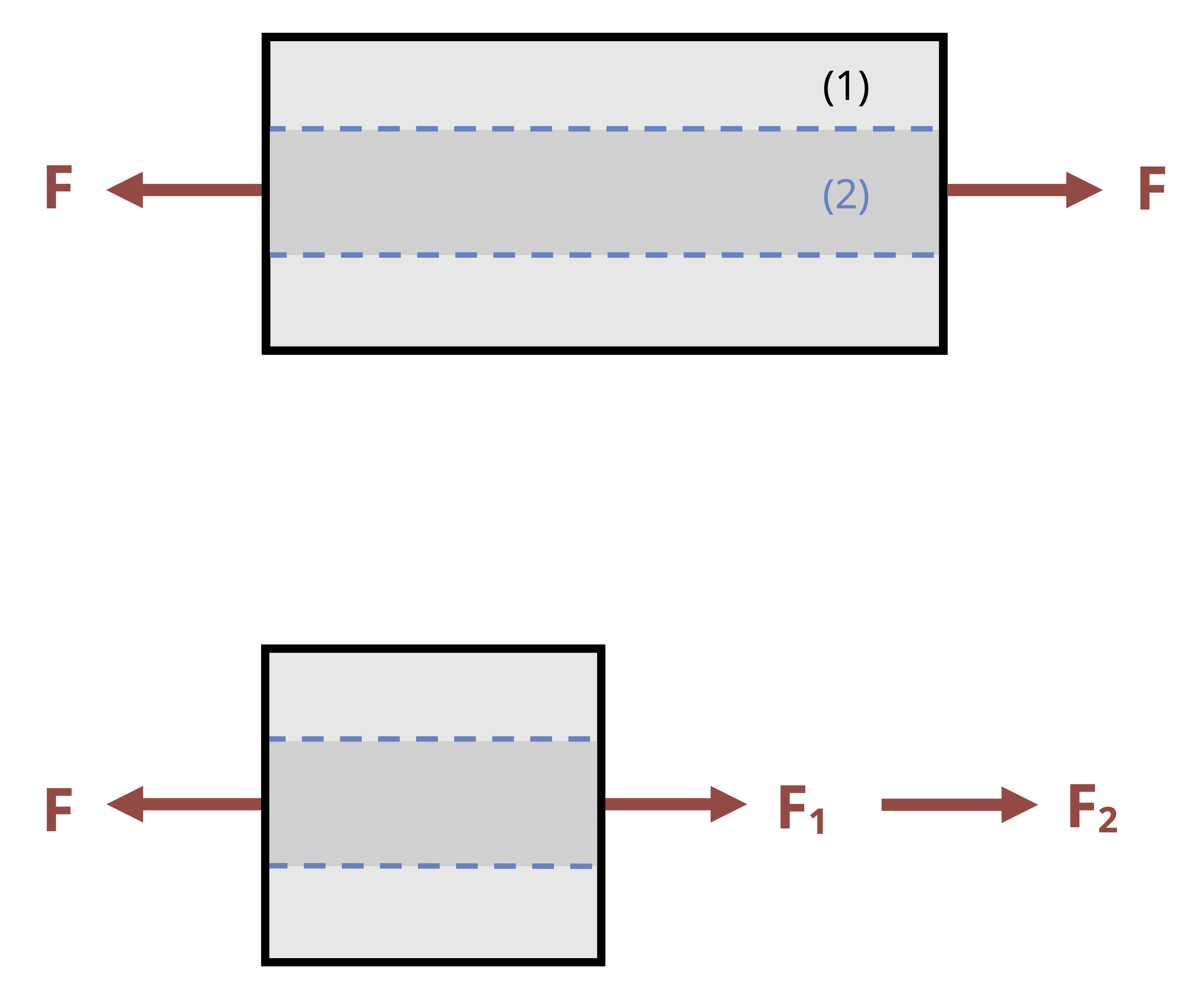
The normal stress discussed in the previous section is averaged over the cross-section and assumes that stresses (and therefore strains) at the cross-section are uniform. In reality stresses and strains can vary across a cross-section, especially if the cross-section is close to an applied load, a support, or a change in geometry. At these points localized stress concentrations occur, leading to large, localized stresses and strains. The intensity of these concentrations depends on the type of loading, support, or geometry (Figure 5.2).
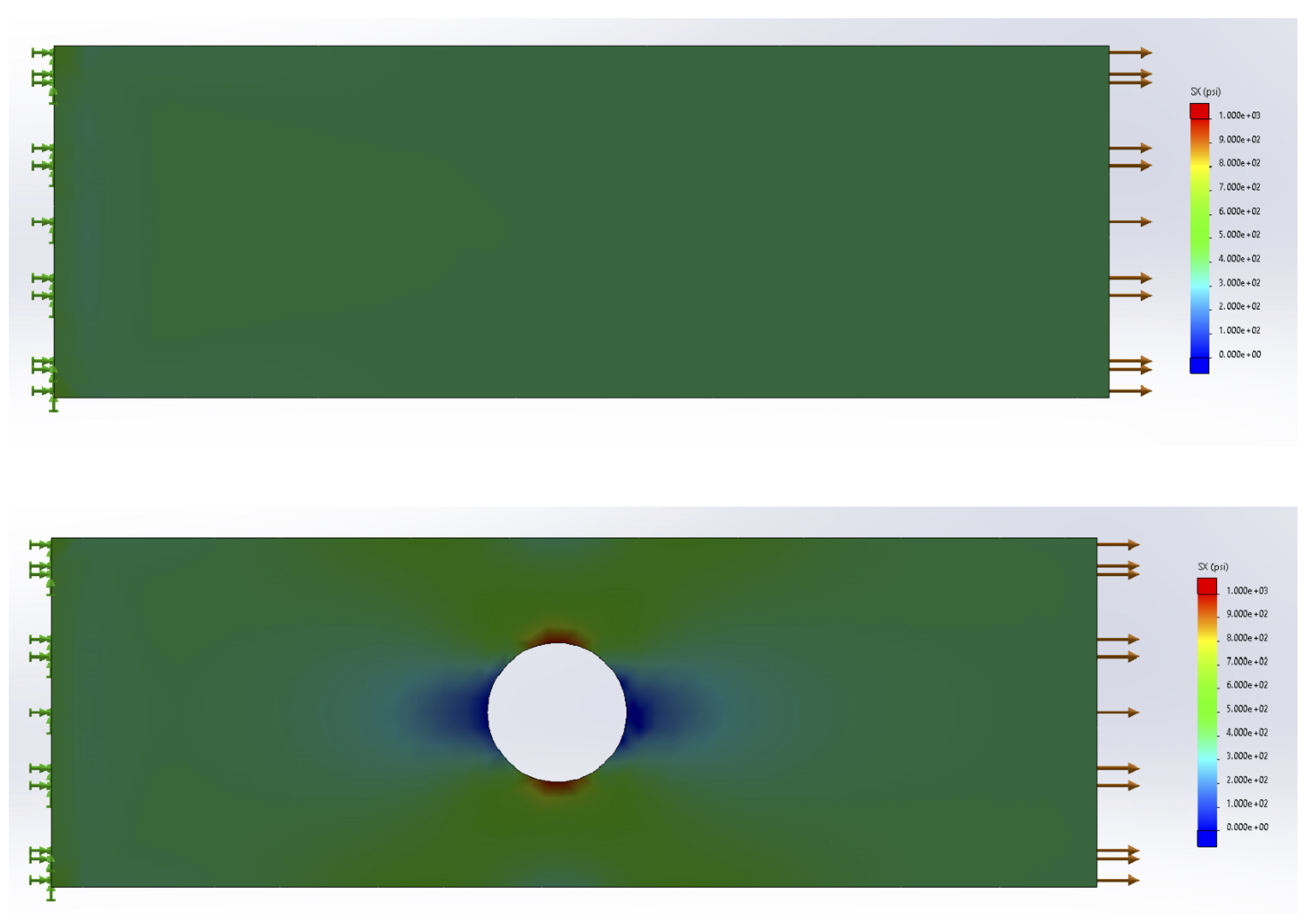
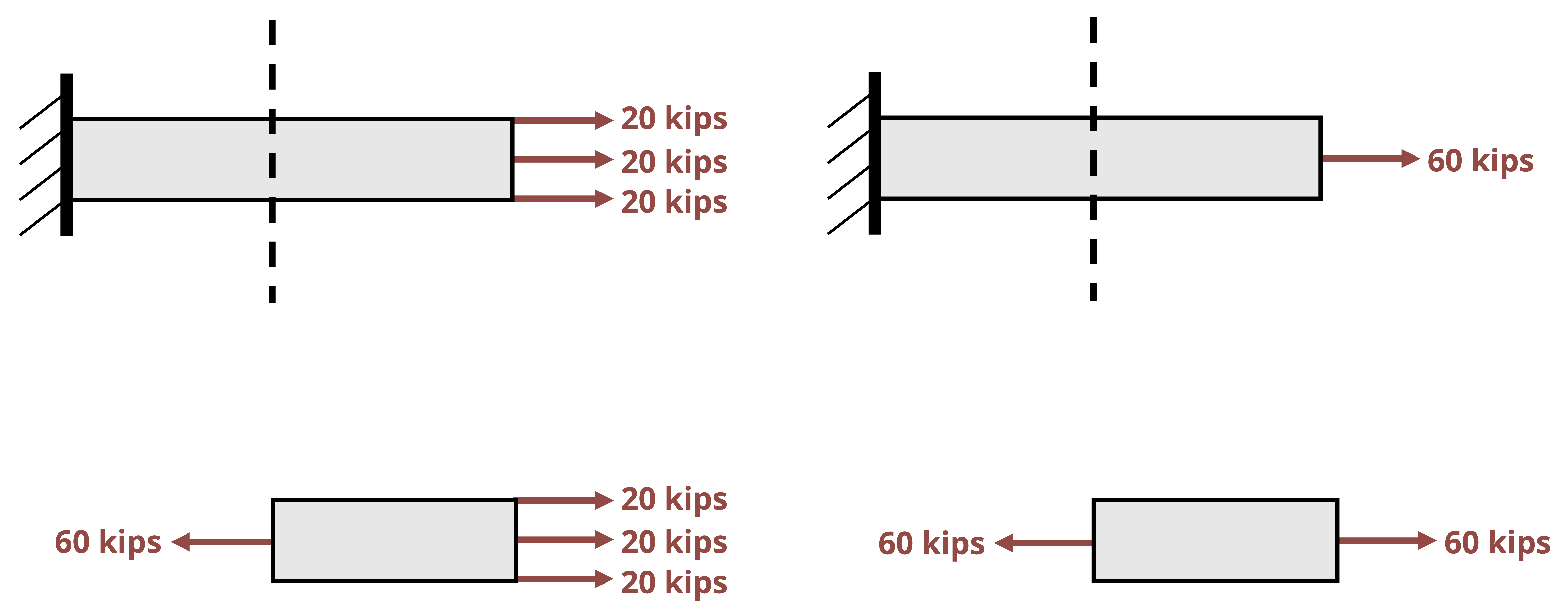
However, these effects disappear a certain distance away from the force, support, or local geometry. It is therefore acceptable to assume uniform stress and strain (as we have been so far) provided that we also assume our cross-section is a sufficient distance away from these points. This is known as Saint-Venant’s principle, which can be formally stated as “The stresses and strains created at a point in a body by two statically equivalent loads are equivalent at points sufficiently far removed from the applied load” (Figure 5.3).
More advanced courses will use the theory of elasticity to study the areas of variable stress and strain, but for now we’ll continue to apply Saint-Venant’s principle and assume that our cross-sections are sufficiently far away from the applied loads that we don’t need to consider these stress concentrations. We will however address the question of stress concentrations around changes in geometry here. We’ll study two specific examples; holes and fillets. Figure 5.2 shows an example of the stress concentrations around a hole. Figure 5.4 shows an example of the stress concentrations around a fillet. A fillet is a rounded corner used to help transition between two geometries.
Fully modeling these stress concentrations is very complicated, but for our purposes it is sufficient to find only the maximum stress that occurs around these stress concentrations. These can be significantly larger than the average stress we have been calculating, and can cause localized failure even if the average stress is below the yield stress for the material. The maximum stress can be found simply by multiplying the average stress by a stress concentration factor, K.
\[ \boxed{\sigma_{max}=K \sigma_{avg}} \tag{5.1}\]
𝜎max = Maximum normal stress [Pa, psi]
K = Stress concentrtion factor
𝜎avg = Average normal stress [Pa, psi]
This stress concentration factor depends on the geometry at hand and can be found from curves in design handbooks (Figure 5.5). See Example 5.1 and Example 5.2 to see how these curves can be used.
Example 5.1
A hole is drilled through a steel plate to allow two components to be bolted together. The plate has the dimensions shown and is 15 mm thick. If the plate is subjected to an axial load of P = 50 kN, determine the maximum stress in the plate if the hole diameter d = 20 mm.
Start by calculating the average normal stress in the plate at the location of the hole. The cross-section is a rectangle with a base of 15 mm (0.015 m) and a height of 100 mm (0.1 m), with a 20 mm (0.02 m) diameter hole cut out.
\[ \sigma_{a v g}=\frac{N}{A}=\frac{50000{~N}}{0.015{~m} *(0.1-0.02){~m}}=41.7{~MPa} \]
Determine the ratio \(\frac{d}{D}\) where d = hole diameter and D = Height of the cross-section. Use the appropriate stress concentration curve to read off the stress concentration factor K for this geometry.
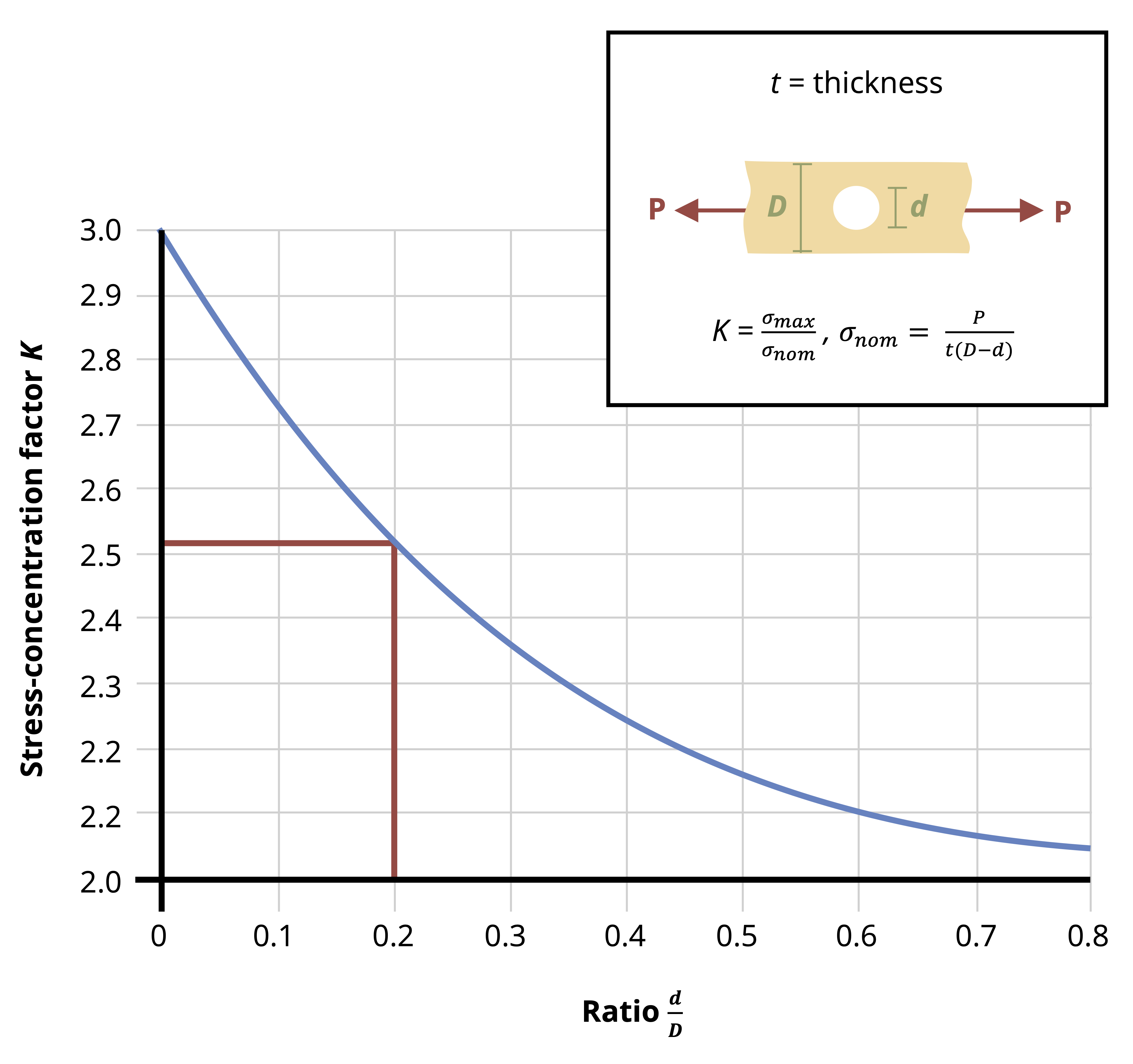
\[ \begin{aligned} &\frac{d}{D}=\frac{20{~mm}}{100{~mm}}=0.2\\ &K=2.525 \end{aligned} \]
Calculate the maximum stress.
\[ \sigma_{max }=K \sigma_{avg}=2.525*41.7{~MPa}=105{~MPa} \]
Example 5.2 A 1-inch-thick connecting rod in an engine assembly has the dimensions shown. If the maximum allowable stress in the rod is 40 ksi, determine the maximum axial load that may be applied to the rod.
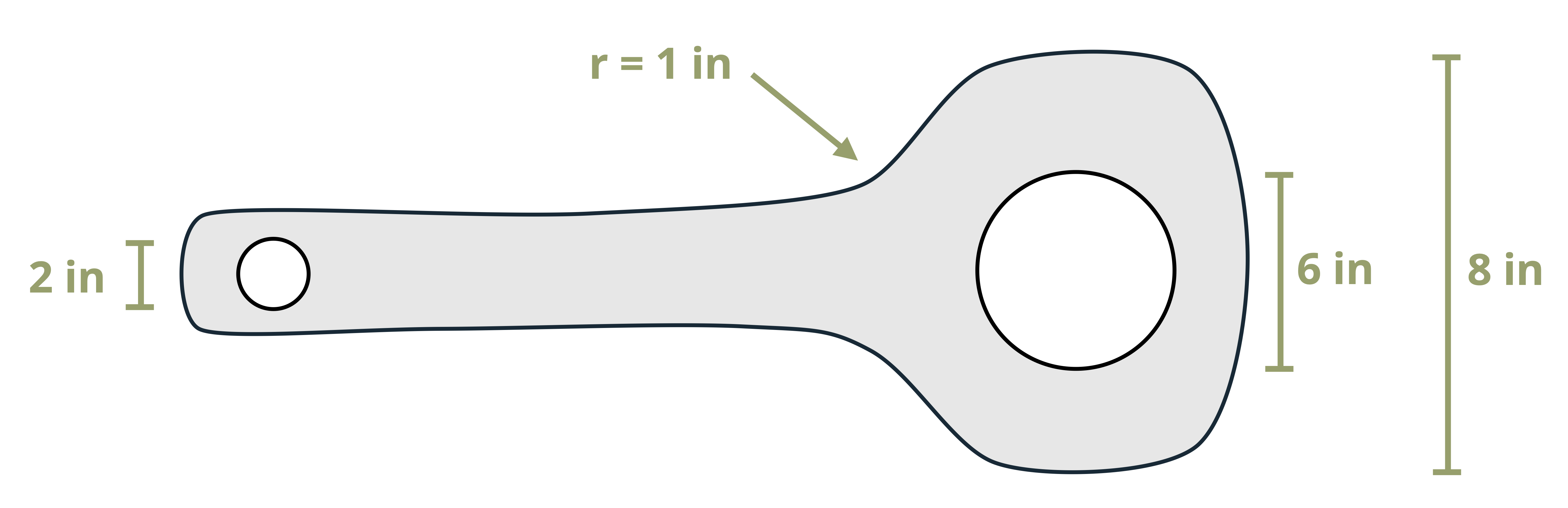
The connecting rod has two holes and a fillet. We can start by determining which of these geometries experiences the largest maximum stress, in terms of applied load P. For each geometry, calculate the average normal stress and then use the appropriate stress concentration curve to determine the maximum normal stress.
For the smaller circle:
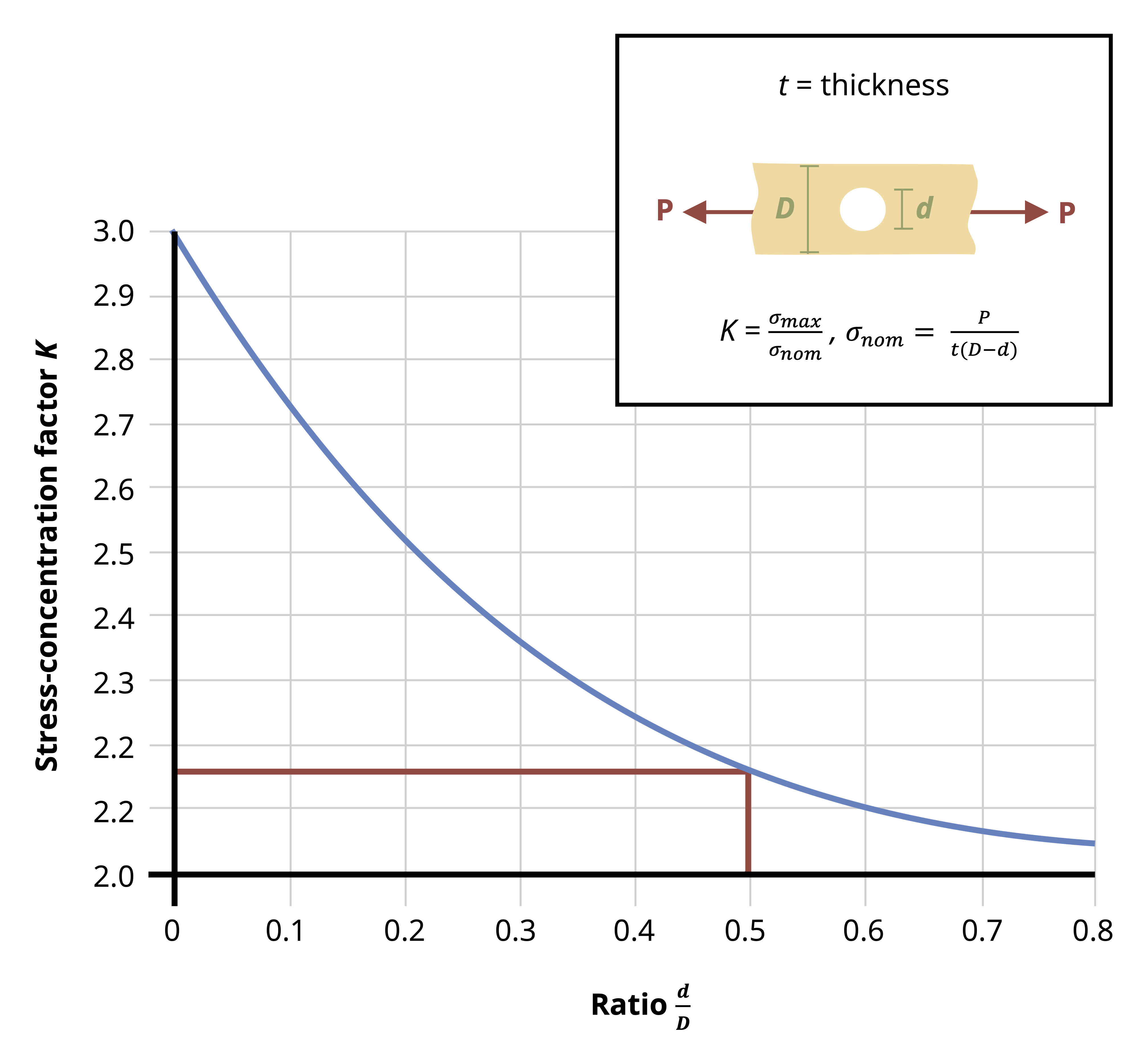
\[ \begin{aligned} & \sigma_{avg}=\frac{N}{A}=\frac{P}{1 *(4-2)}=\frac{P}{2}=0.5 P \\ & \frac{d}{D}=\frac{2{~in.}}{4{~in.}}=0.5 \\ & K=2.15 \\ & \sigma_{max }=K \sigma_{avg}=2.15 * 0.5 P=1.075 P \end{aligned} \]
For the larger circle:
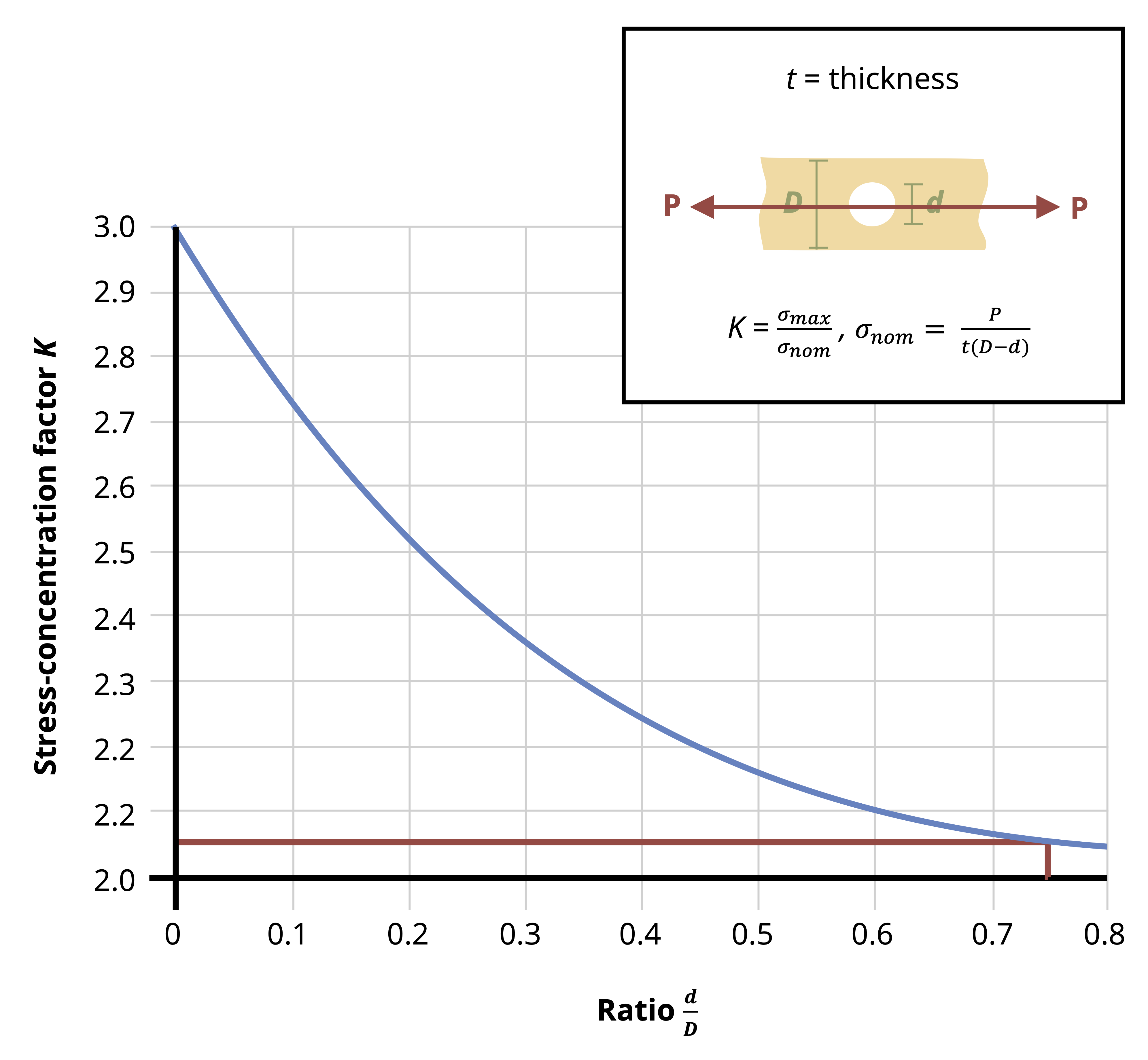
\[ \begin{aligned} & \sigma_{avg}=\frac{N}{A}=\frac{P}{1 *(8-6)}=\frac{P}{2}=0.5 P \\ & \frac{d}{D}=\frac{6{~in.}}{8{~in.}}=0.75 \\ & K=2.05 \\ & \sigma_{max}=K \sigma_{avg}=2.05 * 0.5 P=1.025 P \end{aligned} \]
For the fillet:
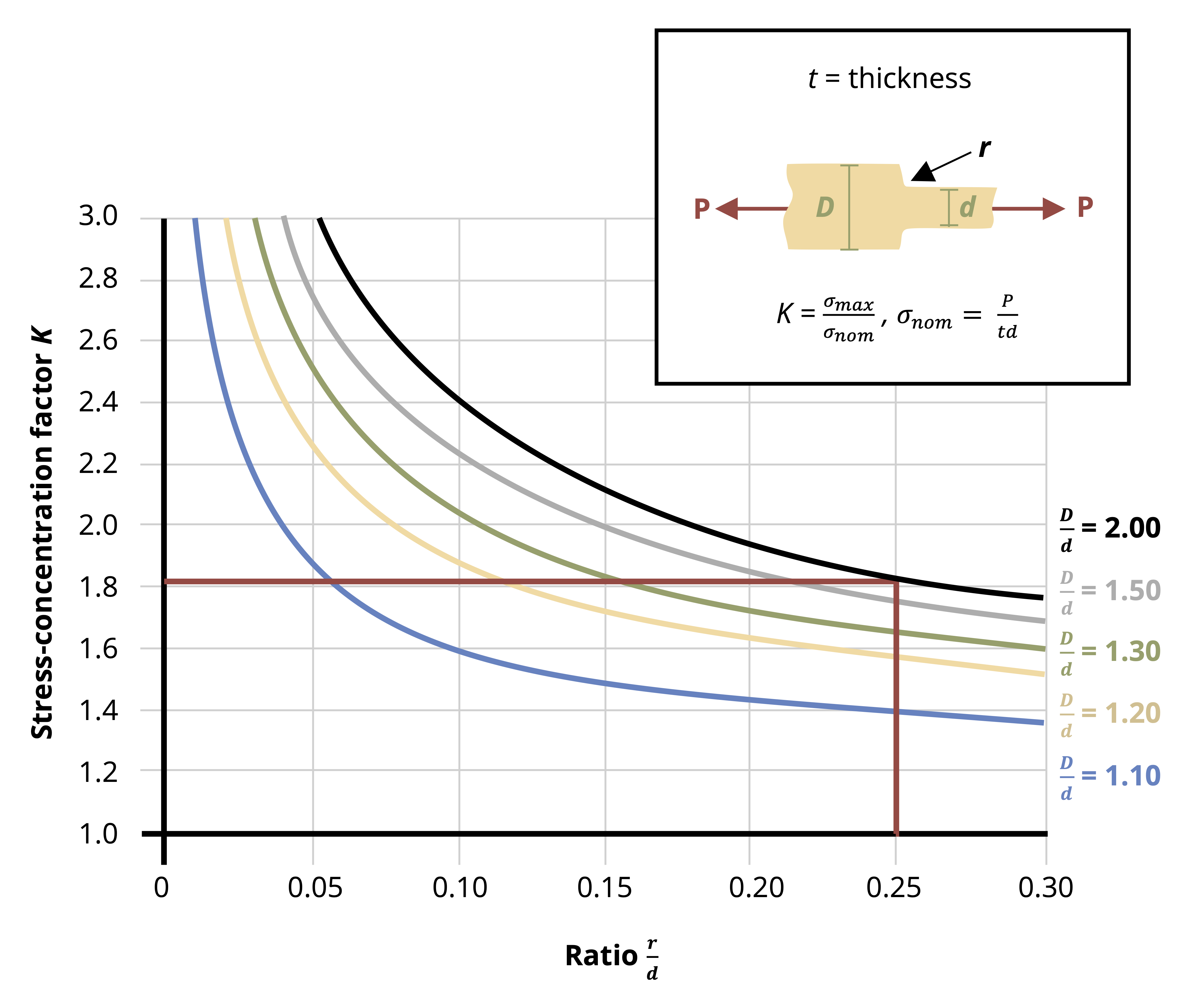
\[ \begin{aligned} & \sigma_{avg}=\frac{N}{A}=\frac{P}{1 * 4}=\frac{P}{4}=0.25 P \\ & \frac{D}{d}=\frac{8{~in.}}{4{~in.}}=2 \\ & \frac{r}{d}=\frac{1{~in.}}{4{~in.}}=0.25 \\ & K=1.82 \\ & \sigma_{max}=K \sigma_{avg}=1.82 * 0.25 P=0.455 P \end{aligned} \]
The largest stress is at the small hole, where 𝜎max = 1.075P.
Since the maximum allowable stress is 40 ksi, \(40{~ksi}=1.075 P \quad\rightarrow\quad P=\frac{40{~ksi}}{1.075}=37.2{~kips}\)
5.3 Axial Deformation
Click to expand
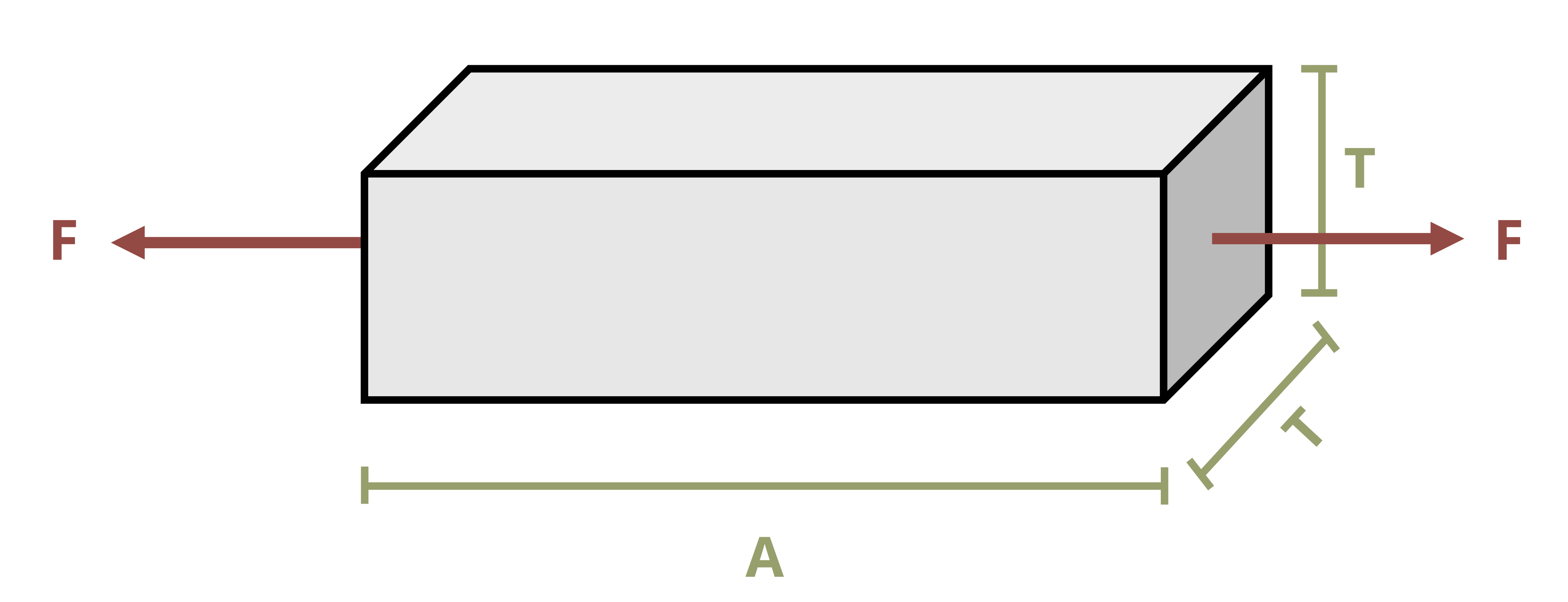
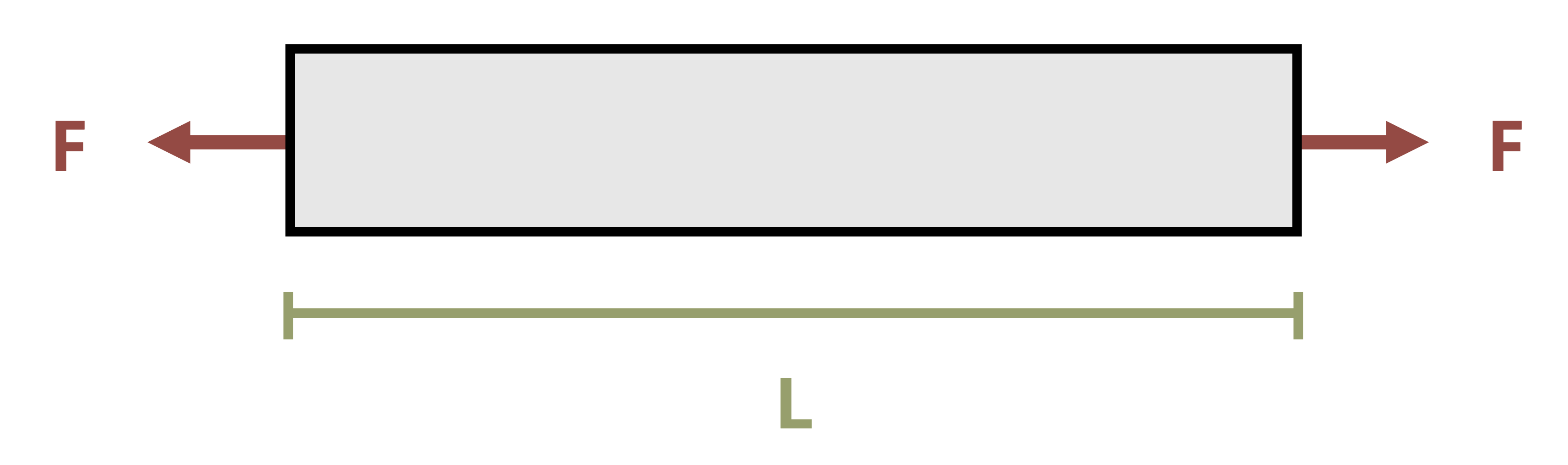
Consider a simple bar of uniform cross-section subjected to an axial force (Figure 5.6).
Assuming elastic behavior, we have equations for stress and strain, as well as Hooke’s law which relates the two equations:
\[ \begin{aligned} & \sigma=\frac{F}{A} \\ & \varepsilon_{long}=\frac{\Delta L}{L} \\ & \sigma=E \varepsilon_{long}\end{aligned} \]
Replacing the stress and strain terms in Hooke’s law:
\[ \frac{F}{A}=E \frac{\Delta L}{L} \]
Rearranging:
\[ \Delta L=\frac{F L}{A E} \]
This equation can be used to directly find the change in length of an object subjected to an axial load.
In practice, there may be multiple axial loads applied to the bar. The cross-sectional area may change at different points along the bar, or perhaps there could be different materials with different elastic moduli connected in series to form the bar. In any of these cases we can split the bar into sections where each section has a constant F, A, and E. We can calculate the change in length of each section separately and sum them to find the total. See Example 5.3 for a problem involving multiple segments of a bar.
\[ \boxed{\Delta L=\sum \frac{F L}{A E}} \tag{5.2}\]
ΔL = Change in length [m, in.]
F = internal axial load [N, lb]
L = Original length [m, in.]$
A = Cross-sectional area [m2, in.2]
E = Elastic modulus [Pa, psi]
Example 5.3
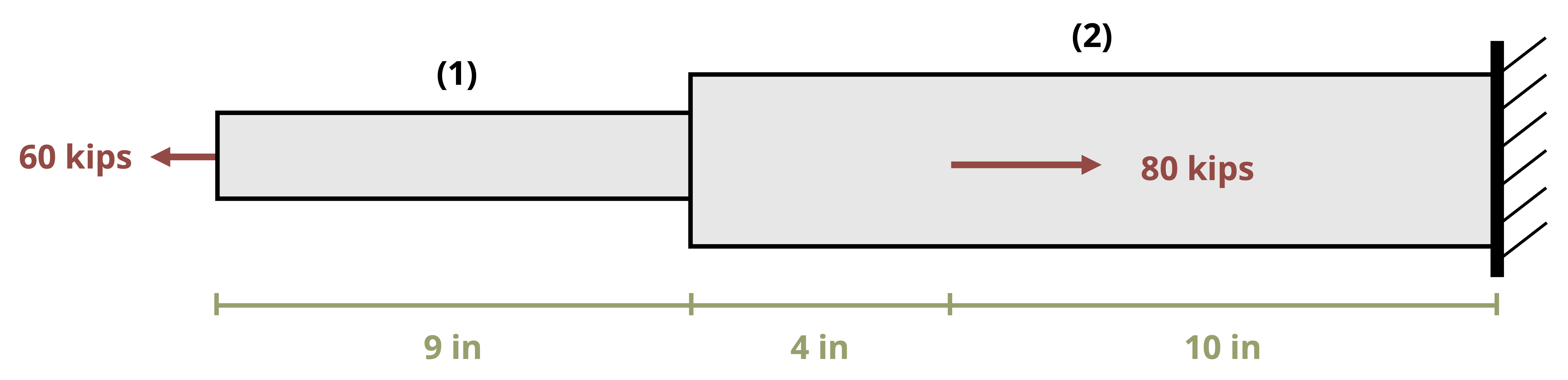
A component is made by welding together 2 circular rods. Rod (1) is made of steel (E = 29 x 106 psi) and is hollow, with an outer diameter of 4 in. and an inner diameter of 2 in. Rod (2) is made of copper (E = 17 x 106 psi) and is solid, with a diameter of 5 in. If the component is subjected to the axial loads shown, determine the total deformation of the component.
We can find the change in length of the component using \(\Delta L=\sum \frac{F L}{A E}\).
First, break the component into three segments and determine the internal load in each segment. The first segment covers the 9-inch steel rod. After the first 9 inches of the component, both the cross-sectional area and elastic modulus change so a second segment is needed. This segment covers the next 4 inches. At this point the loading changes, so a third segment is required to cover the final 10 inches of the component.
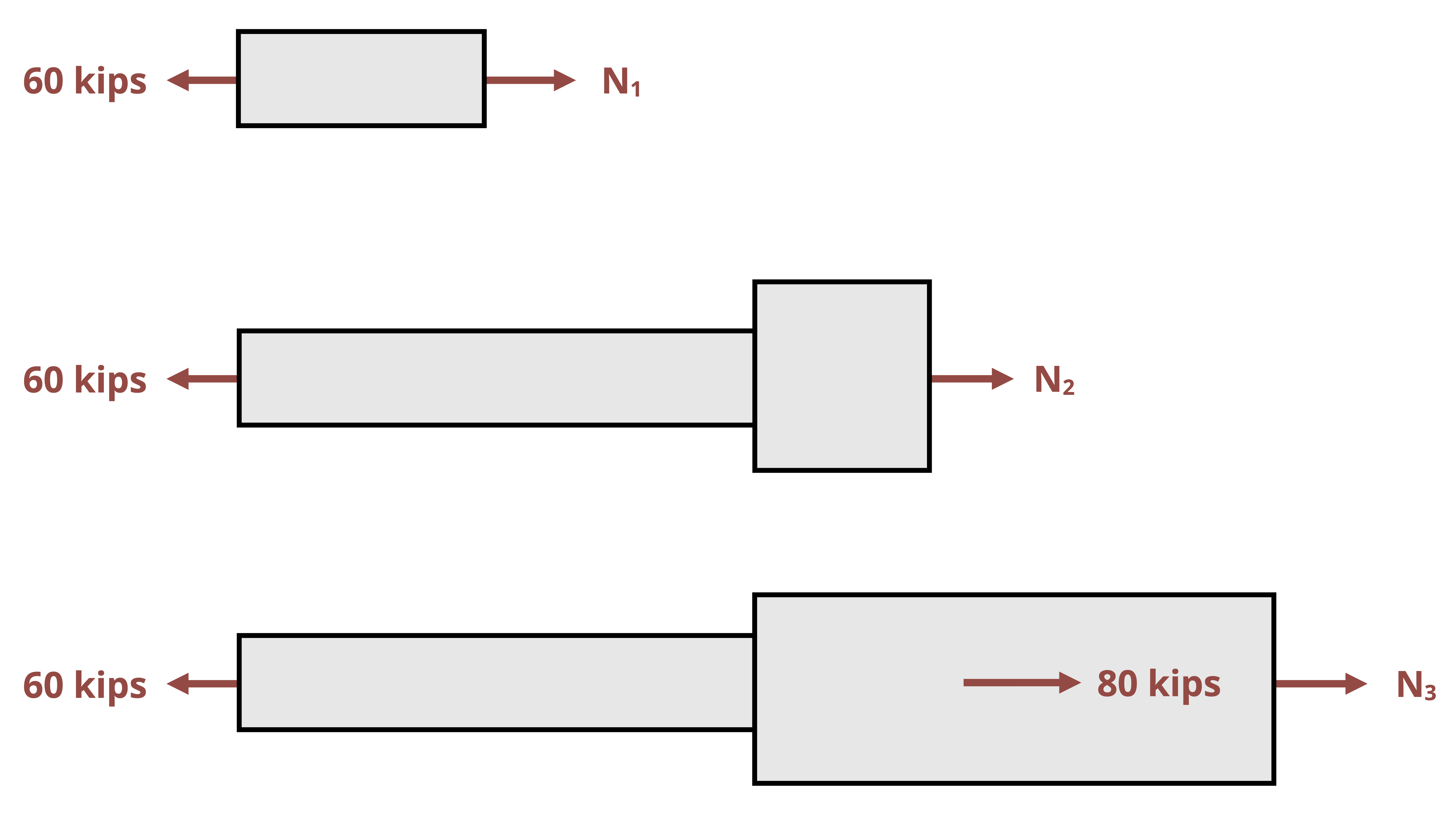
\[ \begin{gathered} N_1=N_2=60{~kips} \\ N_3=-20{~kips} \end{gathered} \]
Now calculate the deformation of each segment. Be sure to use the appropriate dimensions and material properties for each segment.
Cross-sectional areas:
\[ \begin{gathered} A_1=\pi*(2^2-1^2){~in.}^2=9.42{~in.}^2 \\ A_2=\pi*(2.5^2){~in.}^2=19.6{~in.}^2 \end{gathered} \]
Deformation of segment 1:
\[ \Delta L_1=\frac{60000{~lb} * 9{~in.}}{9.42{~in.}^2 * 29 \times 10^6\frac{lb}{in^2}}=0.00198{~in.} \]
Deformation of segment 2:
\[ \Delta L_2=\frac{60000{~lb} * 4{~in.}}{19.6{~in.}^2 * 17 \times 10^6\frac{lb}{in.^2}}=0.000719{~in} . \]
Deformation of segment 3:
\[ \Delta L_3=\frac{-20000{~lb} * 10{~in.}}{19.6{~in.}^2 * 17 \times 10^6\frac{lb}{in.^2}}=-0.000599{~in.} \]
Note that segment 3 is in compression and so gets shorter, while segments 1 and 2 are in tension and so get longer. The total deformation in the component is simply the sum of these three deformations.
\[ \Delta L=0.00198{~in.}+0.000719{~in.}-0.000599{~in.}=0.002{~in.} \]
5.4 Deformation in Series of Bars
Click to expand
Sometimes a structure will have more than one axially loaded member. In such cases there are multiple bars that will experience a change in length and the amount of deformation won’t necessarily be the same in each member. The deformable members are generally connected by a rigid (nondeformable) beam. These problems generally involve a little geometry alongside our deformation equation (Figure 5.7).
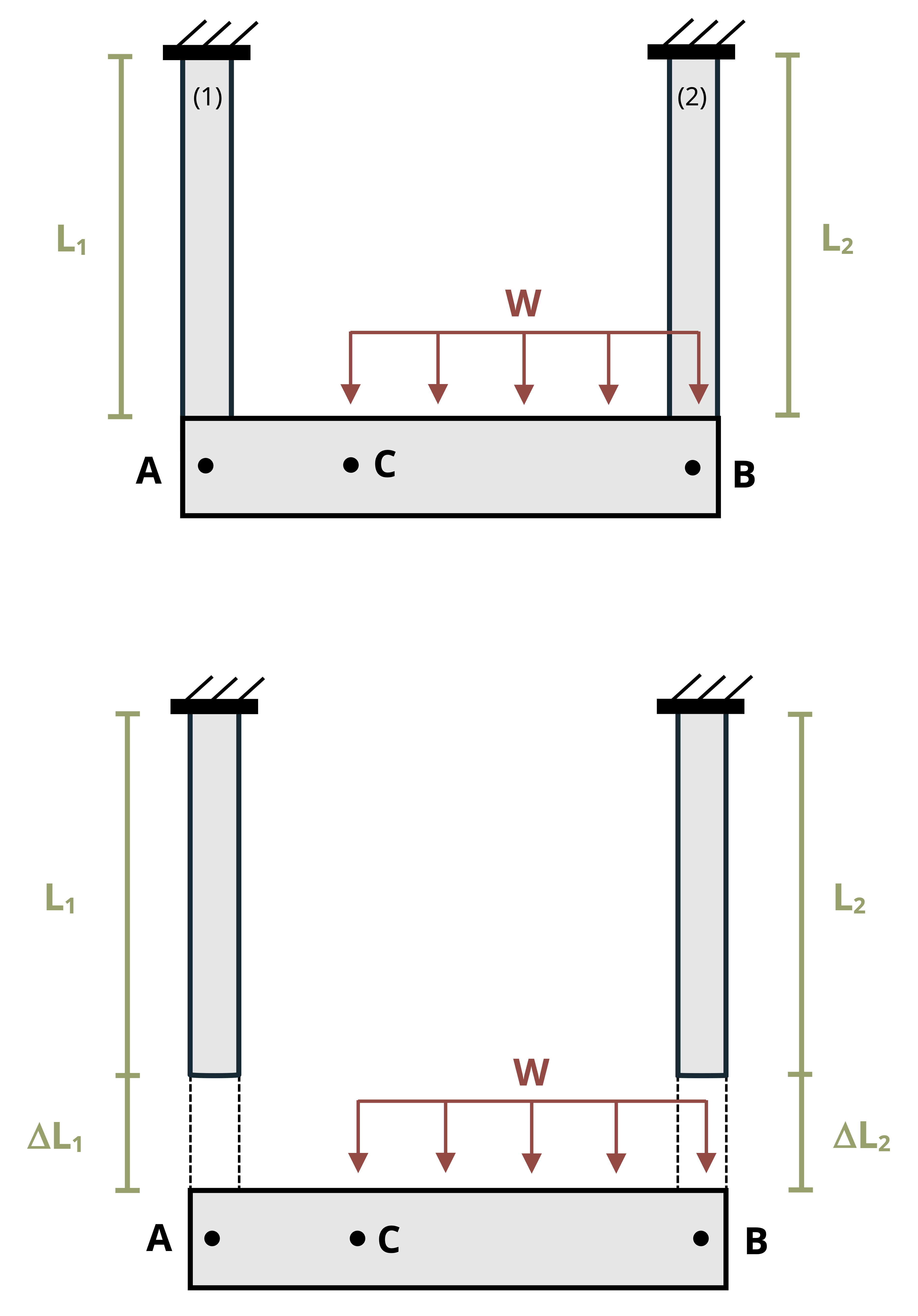
By identifying the force in each member through equilibrium, we may calculate the deformation of each member separately using:
\[ \Delta L=\frac{F L}{A E} \]
Once the change in length of each member is known, we can find the displacement at different points on the rigid beam through simple geometry of the rigid beam (Figure 5.8). This process is demonstrated in Example 5.4.
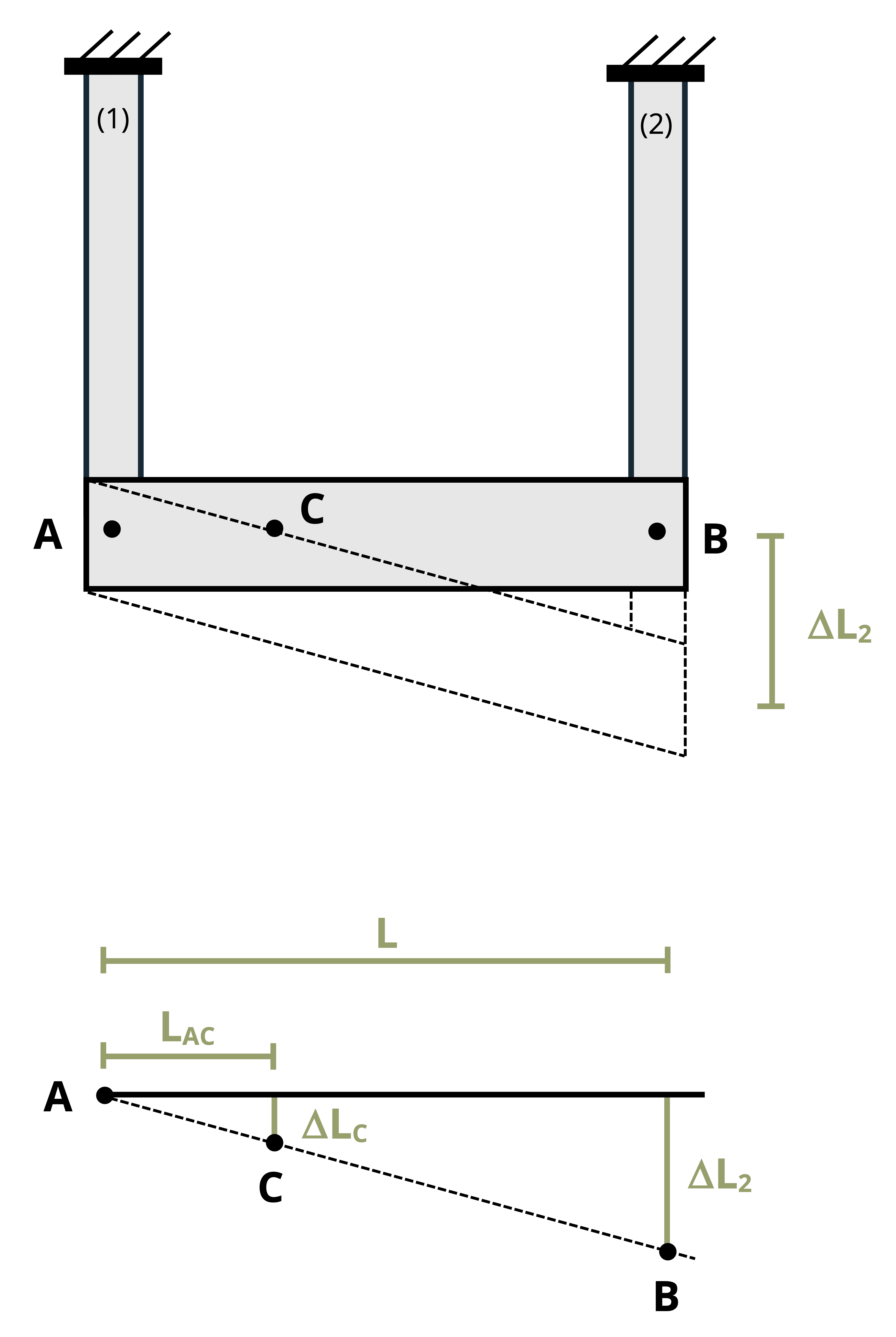
The deflection of point C will be somewhere between the deflection at A and the deflection at B. Assuming there is no deflection at A and assuming that the deflections (and therefore the angle at A) are small, we can use similar triangles to find:
\[ \frac{\Delta L_C}{L_{A C}}=\frac{\Delta L_2}{L} \rightarrow \Delta L_C=\Delta L_2 \frac{L_{A C}}{L}\]
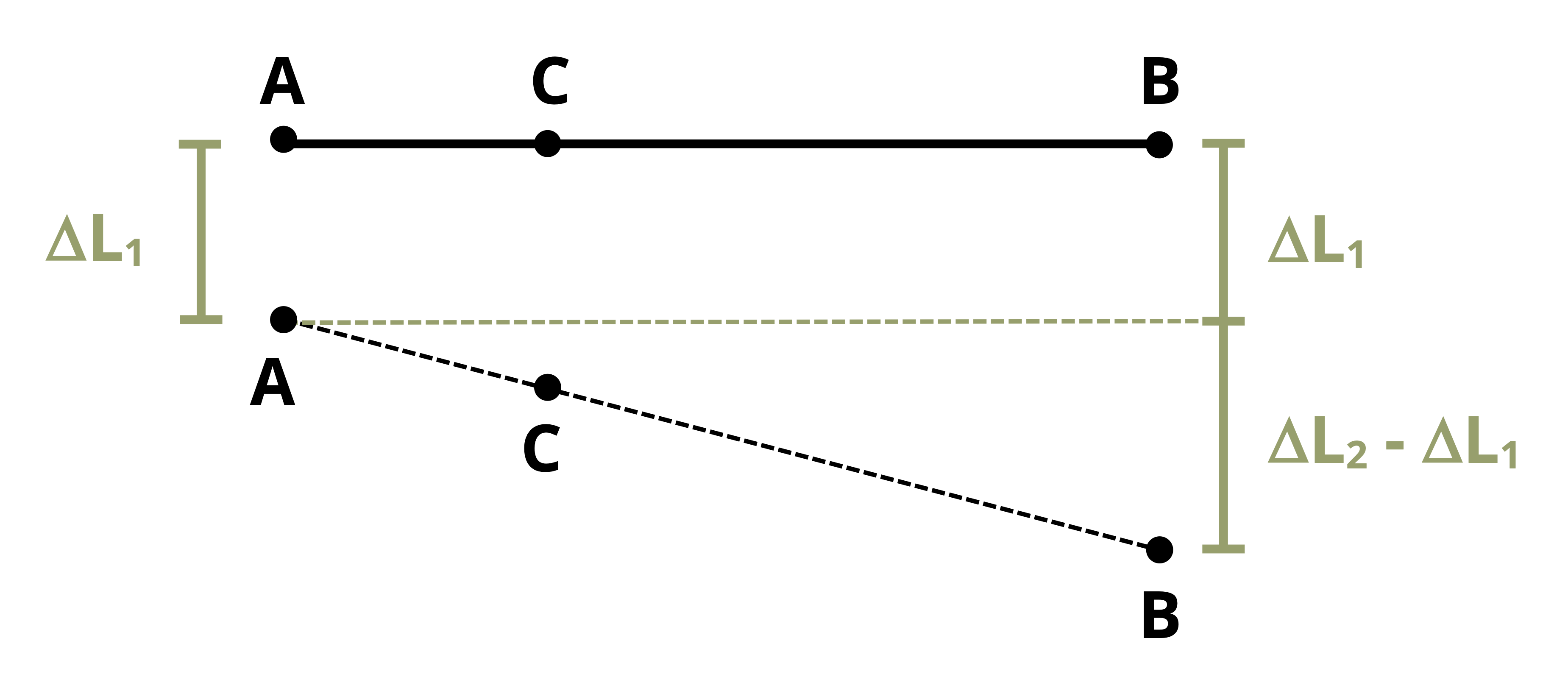
If there is a deflection at point A (Figure 5.9) this simply becomes:
\[ \Delta L_C=\Delta L_1+\left(\Delta L_2-\Delta L_1\right) \frac{L_{A C}}{L}\]
Example 5.4
A rigid beam is supported by two non-rigid poles and subjected to a distributed load w = 75 kN/m. Pole 1 is made of steel (E = 200 GPa) and has a diameter of 30 mm. Pole 2 is made of cast iron (E = 70 GPa) and has a diameter of 50 mm. Determine the deflection at point C of the rigid beam.
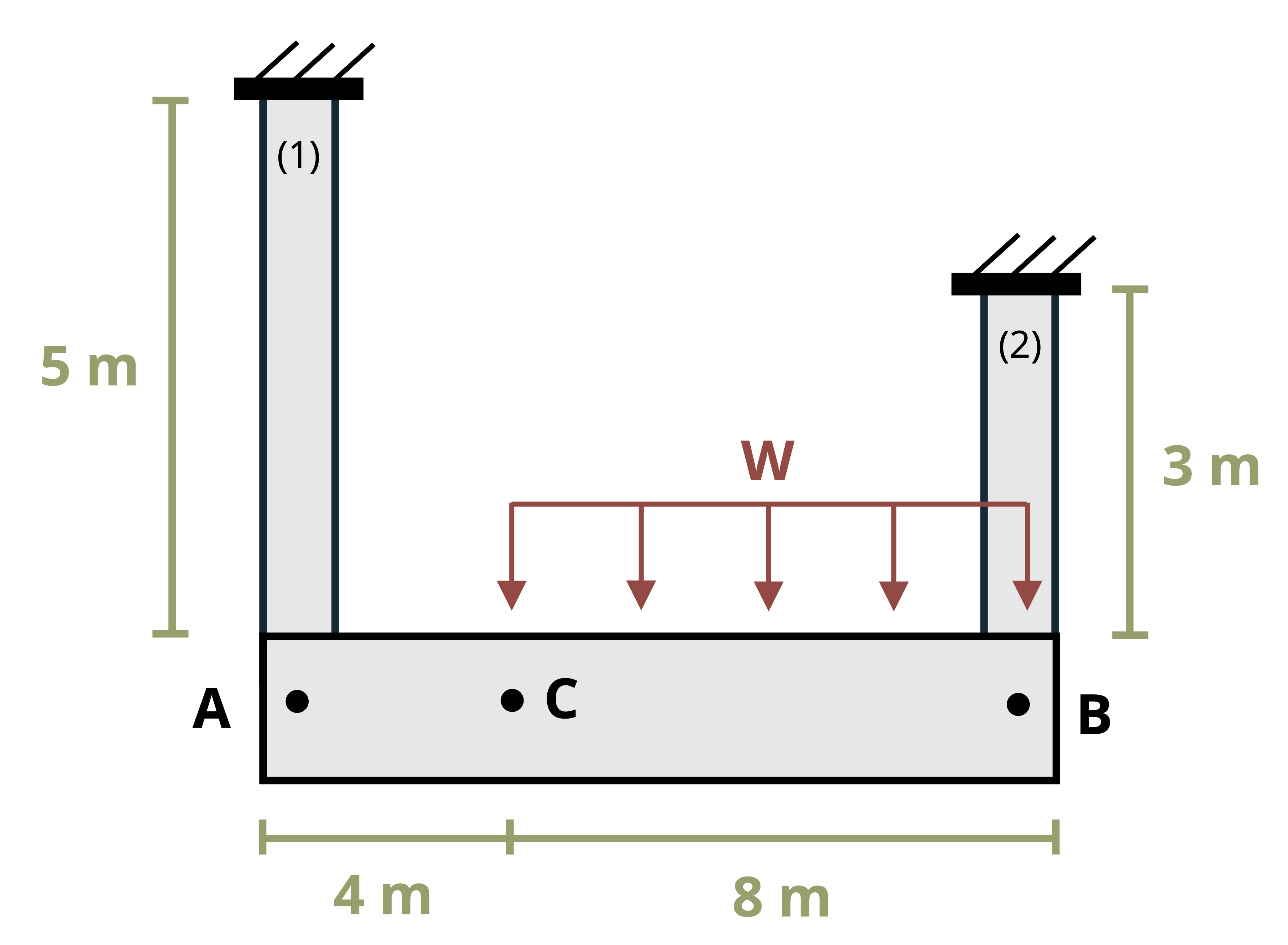
Although the beam is rigid, poles 1 and 2 will both elongate. We can find the force in each pole by drawing a free body diagram and applying equilibrium equations.
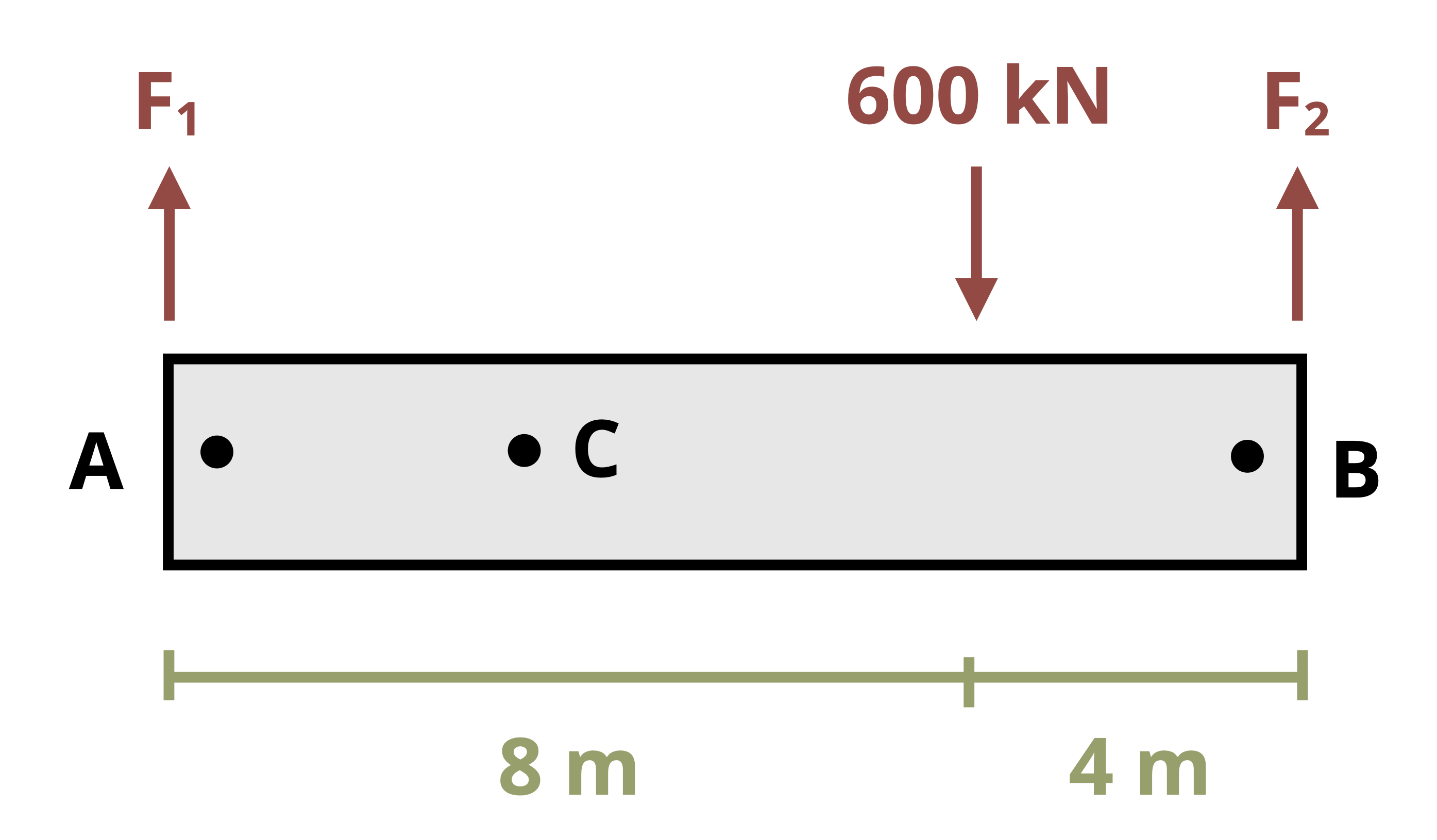
\[ \begin{gathered} \sum M_A=-(600{~kN}* 8{~m})+(F_2 * 12{~m})=0 \quad\rightarrow\quad F_2=400{~kN} \\ \sum F_y=F_1-600{~kN}+400{~kN}=0 \quad\rightarrow\quad F_1=200{~kN} \end{gathered} \]
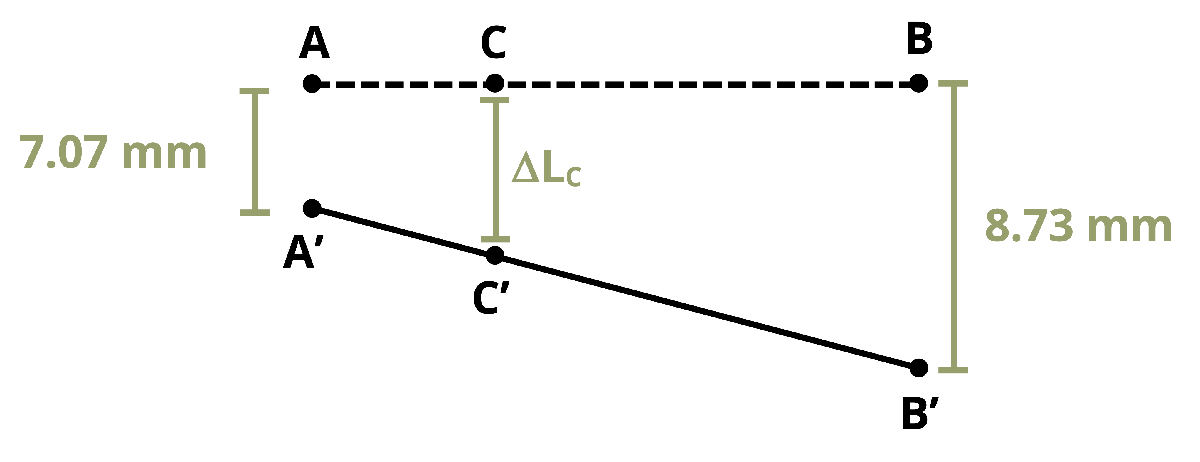
We can then calculate the change in length of each pole.
\[ \begin{aligned} \Delta L_1 & =\frac{F_1 L_1}{A_1 E_1}=\frac{200000{~N} * 5{~m}}{\pi * (0.015{~in.})^2 * 200 * 10^9\frac{N}{m^2}}=0.00707{~m}=7.07{~mm} \\ \Delta L_2 & =\frac{F_2 L_2}{A_2 E_2}=\frac{400000{~N} * 3{~m}}{\pi * (0.025{~in.})^2 * 70 * 10^9\frac{N}{m^2}}=0.00873{~m}=8.73{~mm} \end{aligned} \]
To determine the deflection at point C, first determine that point B has deflected (8.73 mm – 7.07 mm) = 1.66 mm more than point A.
We can find how much more point C has deflected than point A by using similar triangles.
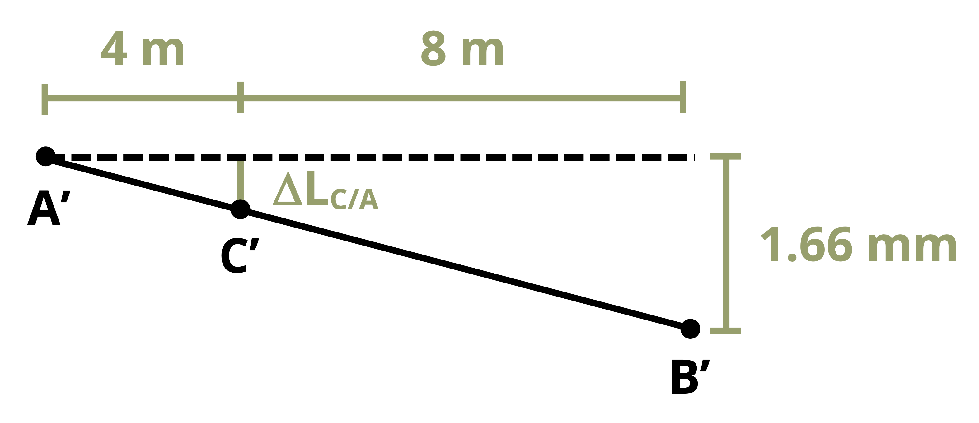
\[ \frac{1.66{~mm}}{12{~m}}=\frac{\Delta L_{C / A}}{4{~m}} \quad\rightarrow\quad \Delta L_{C / A}=0.553{~mm} \]
So point C deflects 0.553 mm more than point A, which is a total deflection at point C of
\[ \Delta L_C=7.07{~mm}+0.553{~mm}=7.62{~mm} \]
5.5 Statically Indeterminate Problems
Click to expand
A statically indeterminate problem is one which has more unknowns than we have equilibrium equations to solve for those unknowns. This is an issue because it prevents us from finding the internal loads and we therefore can’t calculate stress or deformation.
We’ll study two types of statically indeterminate problems. In the first type there will be additional supports beyond those needed to maintain equilibrium. These are known as redundant supports and they are quite common in practice (Figure 5.10).
In such problems, it is not possible to determine all of the reaction forces using equilibrium alone. However, we can use our knowledge of deformation to help. If a member is held between two supports then its total deformation must be zero. Since the change in length depends on the internal force in the member, this introduces an additional equation to use alongside the equilibrium equations. There are two possible approaches here.
Approach 1: To determine the reaction force at the redundant support, begin by removing the redundant support from the problem and determining the deformation that would occur if the support was not there. Then replace the reaction force at the support, which will cause the member to deform in the opposite direction (Figure 5.11).
The sum of these two deformations must equal the actual deformation of the member. If the member is held between two rigid supports, the total deformation will be zero. If there is a small gap or the supports allow a certain amount of movement, the total deformation will be equal to the size of this gap. Example 5.5 shows this process applied to a bar made of 2 materials.
Example 5.5
A 15-foot-tall concrete (E = 4,000 ksi) column has a square cross-section of 6 in. by 6 in. A 10-foot-tall-copper (E = 17,000 ksi) cylinder with an outer diameter of 4 in. and in inner diameter of 3 in. is attached to the top of the concrete. The structure is fixed between two supports. A force of 25 kips is applied as shown. Determine the average normal stress in each material.
To determine the internal force in each material, we first need to find the reaction forces at the supports. We would usually draw a free body diagram and apply equilibrium equations to find these forces. However, this won’t work here because the problem is statically indeterminate.
\[ \sum F_y=F_1+F_2-25{~kips}=0 \quad\rightarrow\quad F_1+F_2=25{~kips} \]
To solve the statically indeterminate problem, remove one of the supports and allow the structure to deform. Either support may be removed. Let’s remove the top support. In this scenario there is no load in the copper cylinder and there is a compressive load of 25 kips in the concrete column.
The total deformation of the structure in this scenario is:
\[ \Delta L=\sum \frac{F L}{A E}=0-\frac{(25{~kips}) *(15 * 12){~in.}}{(6 * 6){~in.}^2 *(4,000)\frac{kips}{in.^2}}=-0.03125{~in} \]
Then replace force F1 and calculate the deformation caused by this force. Since the force is applied at the top of the structure, both the concrete and the copper will elongate.
\[ \Delta L=\sum \frac{F L}{A E}=\frac{F_1 *(10 * 12){~in.}}{\pi(2^2-1.5^2){~in.}^2 *(17,000)\frac{kips}{in.^2}}+\frac{\left(F_1\right) *(15 * 12){~in.}}{(6 * 6){~in.}^2 *(4,000)\frac{kips}{in.^2}} \\ =0.001284F_1+0.00125 F_1 \\ =0.002534 F_1 \]
Since the structure is fixed at both ends, the actual total deformation must be zero.
\[ -0.03125{~in.}+0.002534 F_1=0 \quad\rightarrow\quad F_1=12.3{~kips} \]
Returning to our equilibrium equation, we can also find force F2.
\[ F_1+F_2=25{~kips} \\ 12.3{~kips}+F_2=25{~kips} \\ F_2=12.7{~kips} \]
The internal force in the copper cylinder will be 12.3 kips and the internal force in the concrete column will be 12.7 kips. Finally, calculate the stress in each material. Note from our original free body diagram that the copper cylinder is in tension while the concrete column is in compression. We’ll introduce a negative sign here to indicate compressive stress in the concrete.
\[ \begin{aligned} & \sigma_{copper}=\frac{N_1}{A_1}=\frac{12.3{~kips}}{\pi(2^2-1.5^2){~in.}^2}=2.24 {~ksi} \\ & \sigma_{concrete}=-\frac{N_2}{A_2}=-\frac{12.7{~kips}}{(6 * 6){~in.}^2}=-0.353 {~ksi} \end{aligned} \]
Approach 2: An alternate approach is to start by noting that the total deformation of the bar must be zero. In the case shown in Figure 5.12, we can say that the deformation of segment 1 plus the deformation of segment 2 must add up to zero.
The internal load in segment 1 is FA and the internal load in segment 2 is FB, so there are currently two unknowns. We may use an equilibrium equation to solve for these two unknowns simultaneously.
\[ \begin{aligned} & \frac{F_A L_1}{A_1 E_1}+\frac{F_B L_2}{A_2 E_2}=0 \\ \\ & F-F_A-F_B=0\end{aligned} \]
Example 5.6 re-solves Example 5.5 using this method instead.
Example 5.6
A 15-foot-tall concrete (E = 4,000 ksi) column has a square cross-section of 6 in. by 6 in. A 10-foot-tall-copper (E = 17,000 ksi) cylinder with an outer diameter of 4 in. and in inner diameter of 3 in. is attached to the top of the concrete. The structure is fixed between two supports. A force of 25 kips is applied as shown. Determine the average normal stress in each material.
As before, begin with an equilibrium equation that relates the support loads to the applied load. In this equation we use the convention that forces pointing upwards are positive and forces pointing downwards are negative.
\[ \begin{aligned} & \sum F_y=F_1+F_2-25{~kips}=0 \\ & F_1+F_2=25{~kips} \end{aligned} \]
This bar consists of 2 segments – the copper cylinder (segment 1) and the concrete column (segment 2). Since the bar is held between two rigid supports, the total deformation of these two segments must sum to zero. Note that in this diagram segment 1 is in tension while segment 2 is in compression. We must be consistent with the sign convention that tension is positive and compression is negative.
\[ \frac{F_1 L_1}{A_1 E_1}-\frac{F_2 L_2}{A_2 E_2}=0 \]
Here F1 and F2 are the internal forces in segments 1 and 2 of the bar. These will be the same as the reaction loads at the supports that we are trying to solve for.
\[ \frac{F_1 *(10 * 12){~in.}}{\pi(2^2-1.5^2){~in.}^2 *(17,000)\frac{kips}{in.^2}}-\frac{F_2 *(15 * 12){~in.}}{(6 * 6){~in.}^2 *(4,000)\frac{kips}{in.^2}}=0 \]
Rearrange the equilibrium equation and substitute into the deformation equation.
\[ \begin{gathered} F_1=25{~kips}-F_2 \\ \frac{(25-F_2){~kips} *(10 * 12){~in.}}{\pi(2^2-1.5^2){~in.}^2 *(17,000)\frac{kips}{in.^2}}-\frac{F_2 *(15 * 12){in.}}{(6 * 6){in.}^2 *(4,000)\frac{kips}{in.^2}}=0 \end{gathered} \]
Then simplify and solve for force F2.
\[ \begin{gathered} 0.0321-0.001284 F_2-0.00125 F_2=0 \\ 0.0321=0.002534 F_2 \\ F_2=12.7 {~kips} \end{gathered} \]
Then use the equilibrium equation again to find F1.
\[ F_1=25{~kips}-12.7{~kips}=12.3{~kips} \]
These are the same reactions that we found in Example 5.5 when we solved this problem using the other approach. From here we can find the stress in each material as before, noting again from our diagram that segment 2 is in compression.
\[ \begin{aligned} & \sigma_{copper}=\frac{N_1}{A_1}=\frac{12.3{~kips}}{\pi(2^2-1.5^2){~in.}^2}=2.24 {~ksi} \\ & \sigma_{concrete}=-\frac{N_2}{A_2}=-\frac{12.7{~kips}}{(6 * 6){~in.}^2}=-0.353 {~ksi} \end{aligned} \]
The second type of indeterminate problem involves two materials bonded together in parallel. In these problems it’s possible to find the reactions at the supports, but not possible to find the internal force in each material using only equilibrium (Figure 5.13).
We have one equilibrium equation but two unknown internal forces. However, since the materials are bonded together we can say that they must deform by the same amount. By setting the deformation for each material equal to each other we can define a second equation that involves the two internal forces and, combined with the equilibrium equation, we can now solve for both internal forces. See Example 5.7 for a demonstration.
Example 5.7
A 20-ft-tall concrete (E = 4,000 ksi) column has a square cross-section 6 inches on each side. It is reinforced by six pieces of steel (E = 30,000 ksi) rebar that extend through the length of the column. Each has a diameter of 0.5 inches. The column is subjected to a compressive load of 70 kips. Determine the stress in each material.
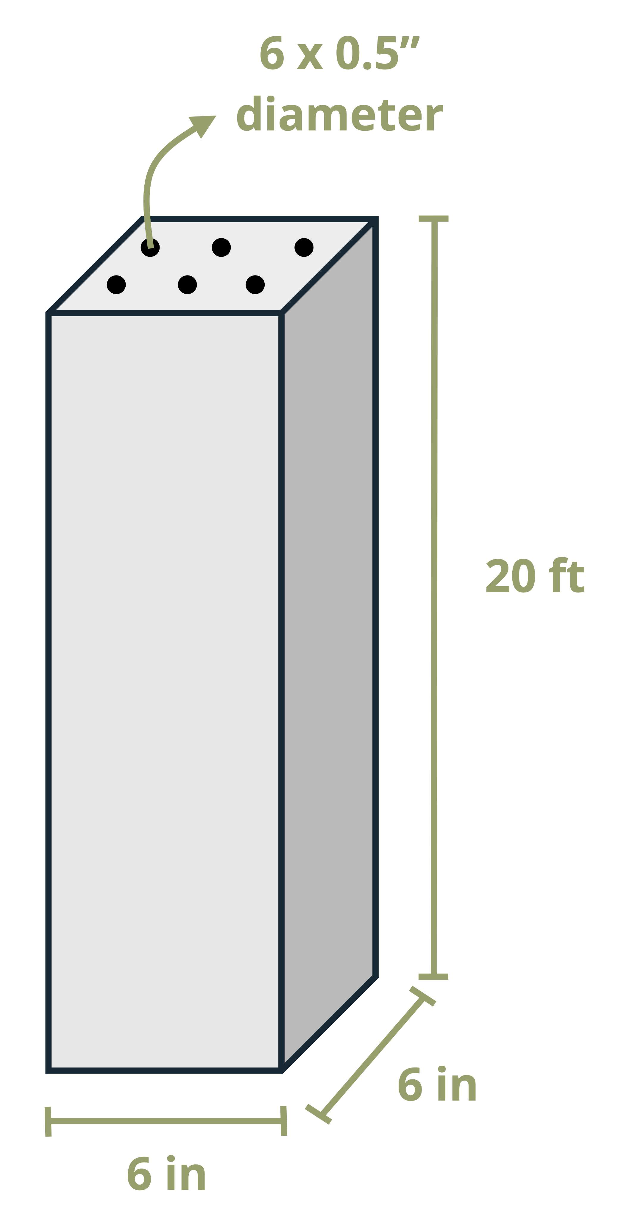
The 70 kips force will be split between the two materials. We need to find the force in each material before we can calculate the stress. Start by cutting a cross-section through the column, drawing a free body diagram, and writing an equilibrium equation.
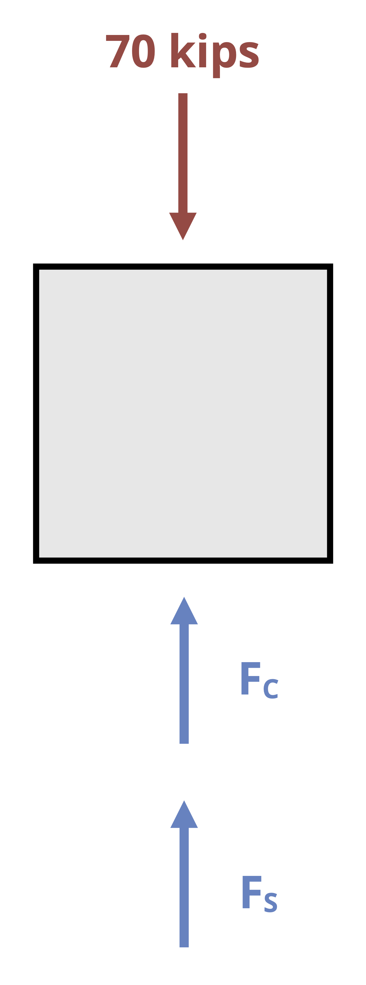
\[ \sum F_y= F_C+F_S=70{~kips} \]
This problem is statically indeterminate, since we have two unknowns and only one equilibrium equation. However, since the two materials are bonded together we can say that they must both deform the same amount.
\[ \Delta L_C=\Delta L_S \]
Since we know \(\Delta L=\frac{F L}{A E}\)
\[ \frac{F_C L_C}{A_C E_C}=\frac{F_S L_S}{A_S E_S} \]
The length of both materials is 20 ft, so this term will cancel.
Although the steel is 6 individual pieces, it’s fine to determine the total area of the steel and the total force in the steel. The total area of the steel is \(A_S=6 * \pi * (0.25{~in.})^2=1.178{~in}^2\)
For the area of the concrete, calculate the area of the square and then remove the area of the 6 rebar rods.
\[ A_C=(6 * 6){~in.}^2-1.178{~in.^2}=34.82{~in.}^2 \]
Substitute these into the deformation equation and rearrange.
\[ \begin{gathered} \frac{F_C}{34.82{~in.}^2 * 4,000{~ksi}}=\frac{F_S}{1.178{~in.}^2 * 30,000{~ksi}} \\ F_C=F_S\left[\frac{34.82{~in.}^2 * 4,000{~ksi}}{1.178{~in.}^2 * 30,000{~ksi}}\right] \\ F_C=3.941 F_S \end{gathered} \]
Substitute this into the equilibrium equation.
\[ \begin{aligned} &F_C+F_S=70{~kips} \\ &3.941 F_S+F_S=70{~kips} \\ &4.941 F_S=70{~kips} \\ &F_S=14.2{~kips} \end{aligned} \]
Then since \(F_C=3.941 F_S \quad\rightarrow\quad F_C=3.941 * 14.2{~kips}=55.8{~kips}\)
Now that we know the force in each material, we can calculate the stress in each material.
\[ \begin{aligned} & \sigma_S=\frac{14.2{~kips}}{1.178{~in.}^2}=12.0{~ksi} \\ & \sigma_C=\frac{55.8{~kips}}{34.82{~in.}^2}=1.60{~ksi} \end{aligned} \]
5.6 Thermal Deformation
Click to expand
So far, we’ve studied the effects of axial forces on an object and how they create stresses and deformations. Temperature changes will also cause an object to deform. As seen in Section 4.6, the strain due to temperature can be predicted by:
\[ \varepsilon_T=\alpha \Delta T \]
As before, strain is dimensionless. The coefficient of thermal expansion is a material constant that can be looked up in handbooks or in Appendix C. Note that for a given change in temperature, the thermal strain will be the same in the axial and transverse directions.
Since strain is also defined as \(\varepsilon=\frac{\Delta L}{L}\), we can also predict the deformation due to a change in temperature:
\[ \varepsilon_T=\alpha \Delta T=\frac{\Delta L}{L} \quad\rightarrow\quad \Delta L=\alpha \Delta T L \]
If the object is free to expand or contract this doesn’t cause any issues and is easy to account for. Many real applications will include a small gap to allow for changes in length due to temperature changes (Figure 5.14). It is even possible that an object is subjected to both a physical force and a temperature change and the total change in length is simply the sum of these effects:
\[ \boxed{\Delta L=\Delta L_F+\Delta L_T=\frac{F L}{A E}+\alpha \Delta T L} \tag{5.3}\]
𝛥L = Change in length [m, in.]
𝛥LF = Change in length due to applied load [m, in.]
𝛥LT = Change in length due to temperature change [m, in.]
F = Internal force [N, lb]
L = Original length [m, in.]
A = Original cross-sectional area [m2, in.2]
E = Elastic modulus [Pa, psi]
𝛼 = Coefficient of thermal expansion \(\left[\frac{1}{^\circ C}, \frac{1}{^\circ F}\right]\)
𝛥T = Change in temperature \([^\circ C, ^\circ F]\)
However if we do not design a gap, or if the gap is not large enough, then the object is not free to expand or contract. As the member pushes or pulls on its supports, a physical force is created. This in turn creates a stress in the object and these stresses can be very large. Such problems are statically indeterminate as the force applied on the member by the support is unknown and can’t be found using only equilibrium. Solving these problems is very similar to solving the first type of statically indeterminate problem. First, remove a support and determine the amount of deformation that would occur due to the change in temperature if the object were free to deform. Then replace the force from the removed support, which will cause the object to deform in the other direction. The sum of these two deformations will equal the total deformation of the member as before. Example 5.8 works through an indeterminate thermal expansion problem.
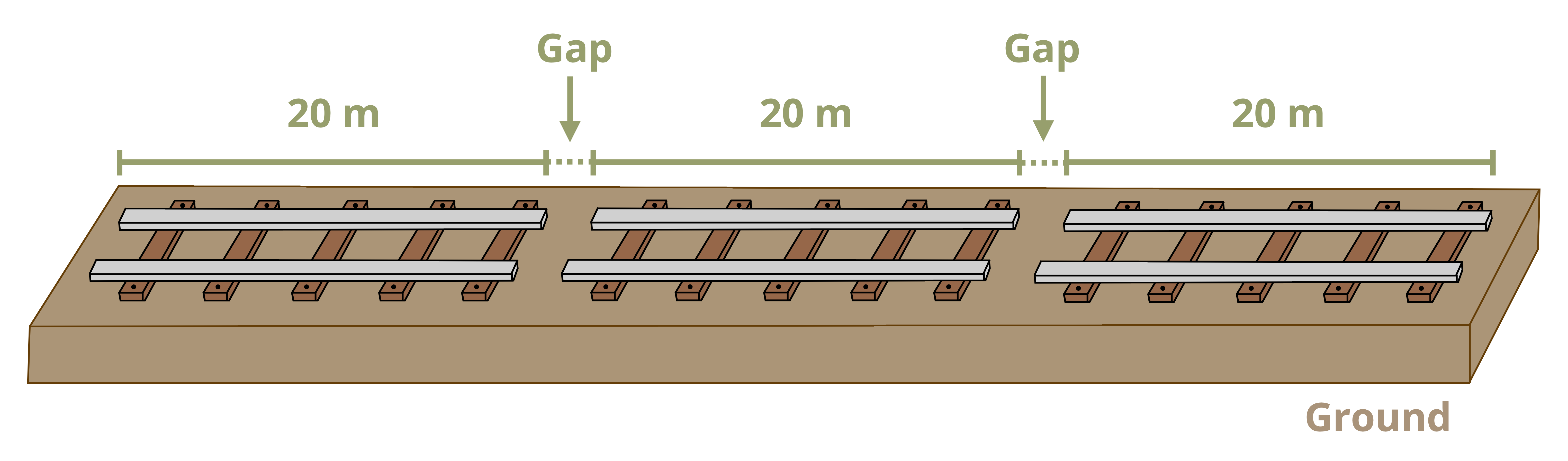
Example 5.8 Steel (E = 200 GPa, α = 11.7 x 10⁻⁶ /°C) train rails are laid end-to-end. Each rail is 20 meters long. A small section of this track is shown below. The rails are laid in winter when the temperature is 0° C. In summer, the maximum temperature is 40°C. Determine the compressive stress in the rail as a result of the temperature change if:
(a) In a particular section of track, the rails are laid with no gap between them.
(b) In another section, the rails have a 5-mm-gap between them.