4 Mechanical Properties of Materials
Introduction
Click to expand
Engineering design of structures meant to carry load often involves the determination of geometries and sizes of the components involved that will be needed to meet the design requirements. Possible design criteria might be that the structure be capable of carrying anticipated loads without failure (e.g., an aircraft wing), that it be stiff enough to only deflect by a limited amount (e.g., a building girder), or that the material returns to its original configuration when the loading is removed (e.g., a 5 MPH bumper). Meeting these criteria requires us to understand the behavior of the material or materials that are being used within the structure. Exploring several of these basic mechanical properties is the focus of this chapter. An understanding of material behavior and these mechanical properties will enable us to relate stresses to strains, temperature change to strains, and explore the coupling that exists when subjecting materials to an arbitrary stress states.
The material properties described in this chapter will vary among materials. Material properties can be measured and recorded for reference in engineering handbooks. Some useful material properties for common engineering materials are recorded in Appendix C.
For the purposes of this book as we learn the principles, we assume that mechanical properties are constant, i.e. independent of temperature, rate of loading, etc.. This assumption works well for many engineering materials such as steel and aluminum at moderate temperatures, but temperature and rate dependence can be important at very high temperatures. Polymers, including plastics, rubber, etc. are known for their significant temperature and time or rate dependence, sometimes at common use temperatures, complicating the ability to tabulate these properties in a simple table. Practicing engineers often need to recognize and address such complications as they work with such materials.
Of particular importance is that materials in this text are assumed to be isotropic—that is, they have the same properties when loaded in different directions. Anisotropic materials, which display different properties depending on the direction of loading, are quite common but are beyond the scope of this text.
Section 4.1 discusses a common method of determining mechanical properties, known as the Tensile Test. The output of the Tensile Test - the Stress-Strain Diagram - is analyzed in Section 4.2.
Important mechanical relationships Hooke’s Law, which relates stress to strain, and Poisson’s ratio, which relates normal strain in the axial and lateral directions, are covered in Section 4.3 and Section 4.4.
Section 4.5 considers the relationship between shear stress and shear strain and Section 4.6 introduces the concept of thermal strain. In Section 4.7 we expand Hooke’s Law from Section 4.3 to the general three-dimensional case.
Finally, in Section 4.8, we consider applying a factor of safety to our designs to ensure they don’t fail.
4.1 Tensile Test
Click to expand
A common method of measuring mechanical properties of materials is the tensile test, which involves placing a cylinder or bar of material in a load frame (such as shown in Figure 4.1 (A)) and subjecting the specimen to tensile loading. These load frames are designed in such a manner that they can mechanically extend the tensile bar, often to failure, while measuring both the imposed load and the specimen deformation. These quantities for the specimen are then used to determine the local or material level behavior of stress and strain by using the relationships covered in Chapter 2 and Chapter 3. These latter quantities are often essential in engineering design because properties from appropriate tests on laboratory specimens may be used to predict the behavior of much more complex engineering components.
During a typical tensile test, a specimen (such as shown in Figure 4.1 (B)) is mounted in grips that are then separated at a prescribed displacement rate. To determine stress, the recorded force at any time is divided by the cross-sectional area of the specimen. Because of the likelihood of failures at the grip due to concentrations of stress, specimens are typically “waisted” to form dogbone or dumbbell shapes. Large fillets are used to reduce stress concentrations associated with the different areas (See Section 5.2), and failure will typically occur within the narrowed region of the specimen due to the smaller cross-sectional area. This region is often referred to as the “gage region” as this becomes the area of interest for the specimen. In addition, this specimen produces a uniform uniaxial stress state within this gage region of the specimen. The normal stress within this region is determined by:
\[ \sigma=\frac{F}{A} \]
To determine strain, devices such as mechanical extensometer’s (see Figure 4.1 (C)) are mounted on the specimen, measuring the deflection and dividing it by the original distance between the contact points. The axial normal strain is determined by dividing the measured extension by the active length of the strain measuring device, typically a portion of the gage section of the specimen:
\[ \varepsilon=\frac{\Delta L}{L} \]
4.2 Stress/Strain Diagram
Click to expand
The goal in conducting tests of materials, such as the tensile test described above, is to learn qualitatively how the specimen responds and to quantitatively determine important mechanical properties of the material.
As discussed in the introduction to this chapter, these material properties will be assumed to be constant in this text and so, once determined from a test specimen, can be used to design and analyze components made of that same material. Appendix C contains material properties for a selection of these materials.
Figure 4.2 (A) illustrates representative stress-strain behavior for several engineering materials.
Each material initially experiences a linear relationship between stress and strain, represented as a straight line on the stress/strain diagram. This linear portion is referred to as elastic deformation. One important property of elastic deformation is that if an object is loaded into the elastic region (causing a certain amount of stress and strain) and the load is subsequently removed, the object will return to its original dimensions.
Materials such as glass, silicon wafers, and concrete tend to be quite brittle, breaking prior to significant permanent or plastic deformation. The behavior remains nearly linear until failure, an attribute of brittle materials. On the other hand, certain copper alloys, mild steel, and many polymers are often quite ductile, meaning that there is considerable plastic deformation beyond some limiting value of stress or strain. Unless a material is perfectly brittle, there will be a certain point beyond which the relationship between stress and strain becomes nonlinear, represented by a curve departing from linear elastic behavior on the stress/strain diagram. This nonlinear (often curved) portion is referred to as plastic deformation. If an object is loaded into the plastic region and the load is subsequently removed, any plastic deformation is permanent, and the object will not return to its original dimensions.
The transition between the linear region of the stress-strain curve and the subsequent behavior marks an important engineering property of the material known as the yield stress. Although considerable variations are seen among different materials, yielding is typically defined as the region within which relatively small increases in stress are associated with relatively large increases in strain. The yield strength of the material is a very important design parameter, as many engineering components are designed to operate within the linear region of material response, and hence remain elastic, i.e., the ability to return to their original configuration when loading is removed. You likely have experienced material yielding if you have ever deformed a coat hanger or paperclip such that it does not return to the original state. Such behavior is undesirable for many engineering components designed to continue operating in their original state. On the other hand, plastic deformation following yielding can be very important in terms of the fabrication process. For example sheets of steel or aluminum can be placed between molds and compressed under high pressure to deform them into the shape of an automobile panel as seen in Figure 4.3 (A), an illustration of where plastic deformation is very important. Plastic deformation can also be useful in absorbing energy, such as seen in the concertina crushing of a structural component for an automobile (see Figure 4.3 (B)). This book, however, will focus on the pre-yield, linear elastic region.
Sometimes the yield region is further described by three distinct points on the stress/strain curve. The proportional limit marks the point where the relationship between stress and strain stops being linear. The elastic limit marks the point beyond which materials do not return to their original state. The yield point is typically defined using the 0.2% offset method where a straight line beginning at a strain of 0.002 (0.2%) and running parallel to the linear portion of the diagram is drawn. The point where this line intersects the stress/strain curve is defined as the yield point. Since these three points for a material often occur within a fairly narrow range of one another, this text will refer to these three points collectively as yielding, and will define the stress at this point as the yield strength. Figure 4.4 illustrates these definitions.
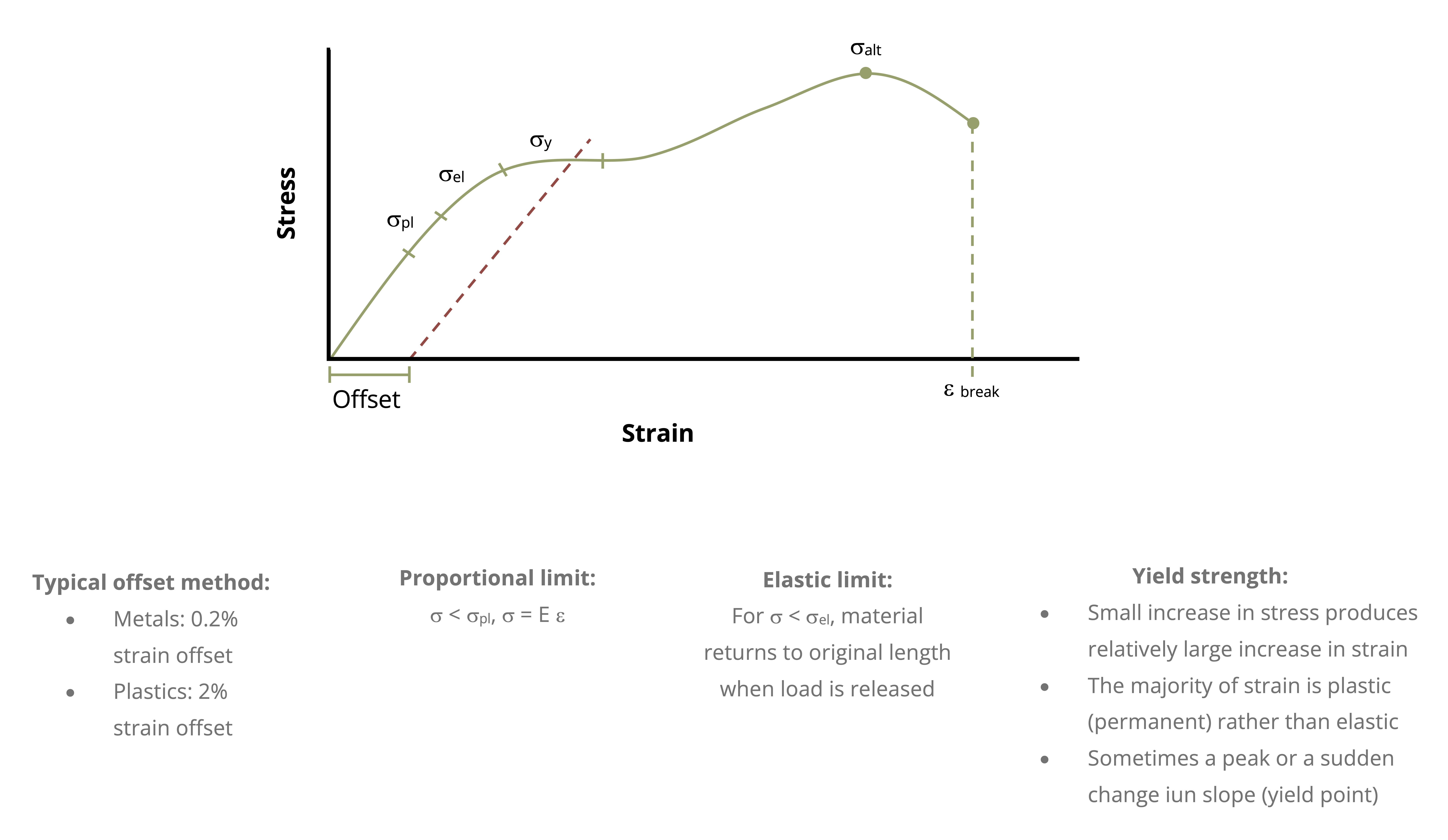
Other metrics are also often quantitatively evaluated from stress-strain diagrams, including the ultimate strength, \(\sigma_{alt}\), the maximum stress achieved prior to failure and the strain at break, \(\varepsilon_{break}\) which is a measure of the ultimate elongation capabilities of the material (though is often dependent on the size of the specimen’s gage length.
4.3 Hooke’s Law
Click to expand
The slope of the linear region of this stress/strain diagram represents an important material property known as Young’s modulus or the modulus of elasticity, which will be designated by E. The elastic modulus can be thought of as a measure of stiffness of the material. A high elastic modulus for ‘stiff’ materials is represented by a steep slope. That is, a large increase in stress with only a small increase in strain. A low elastic modulus for ‘soft’ materials is represented by a shallow slope indicating a small increase in stress but a large increase in strain.
Thomas Young (1773-1829) was a British scientist, who noted the proportionality between applied force and extension, which he recorded as “ut tensio sic vis”, meaning “as is the extension, so is the force”.

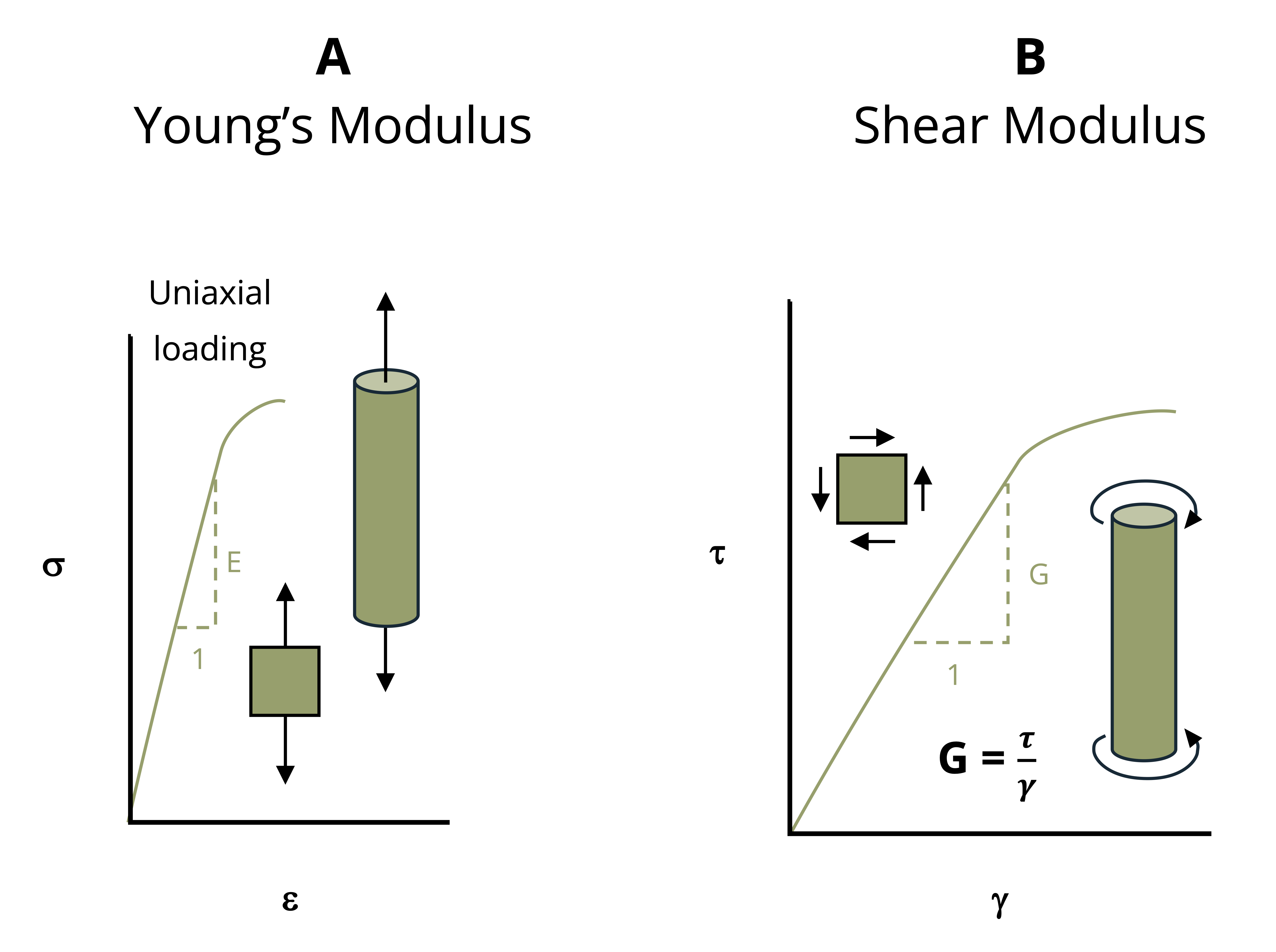
The linear elastic region of material response is of enormous importance for most engineering structures. Loading significantly beyond this proportional limit can result in pronounced yielding and permanent deformation that is often unacceptable, unless one is using this deformation to absorb energy (as in automobile frame involved in collision). Young’s modulus or the modulus of elasticity is illustrated in Figure 4.6 (A), which plots a portion of the normal stress versus normal strain, for example from a tensile test.
\[ E=\frac{\sigma}{\varepsilon} \]
Since strain is unitless, elastic modulus will have the same units as stress [Pa or psi].
This relationship is more commonly called Hooke’s Law, and written in the form:
\[ \boxed{\sigma=E \varepsilon} \tag{4.1}\]
𝜎 = Average normal stress [Pa, psi]
E = Elastic modulus [Pa, psi]
𝜀 = Normal strain
It is especially important to note that this relationship is only applicable within the linear elastic region of the material’s response. Use of this relationship beyond this region can lead to serious design mistakes. One should note that this proportionality, applicable at the material level for stress and strain, also extends to structural elements, such as bars in tension or compression, beam deflections, helical springs in which the force and deflection are related by the spring constant, and many other engineering components and structures, as will be covered in the following chapters of the book.
Example 4.1 uses Hooke’s law to determine the elastic modulus of a material where the applied load and deformation are known.
Example 4.1
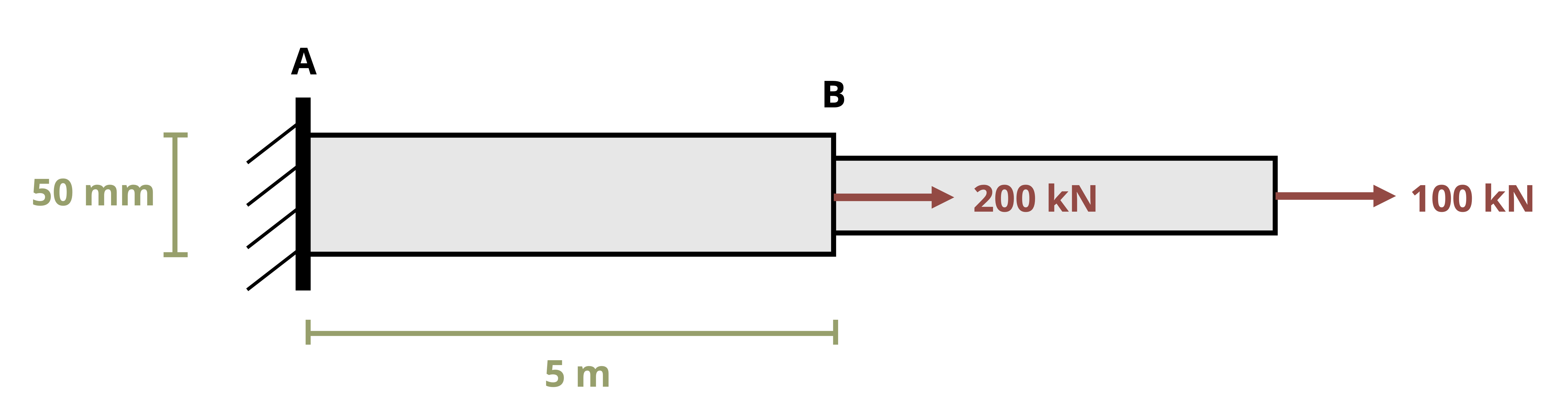
Two bars are welded together and fixed to a wall at A. Two loads are applied as shown. Bar AB is 5 m long and has a diameter of 50 mm. If the change in length of bar AB is 4 mm, determine the elastic modulus of this bar.
Cut a cross-section through bar AB and determine the internal load.
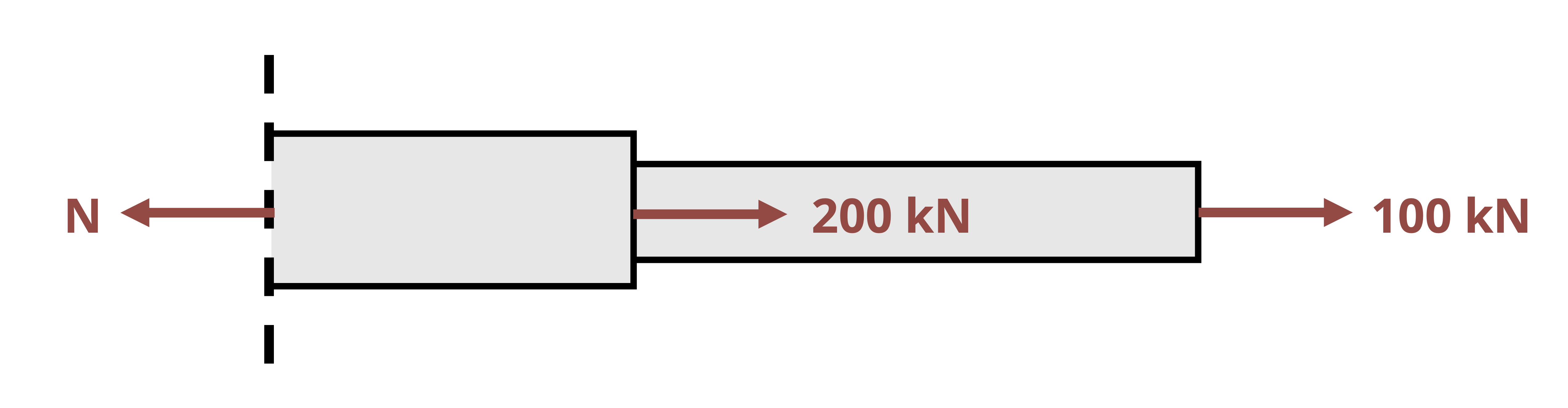
\[ \sum F_x= 100{~kN}+200{~kN}-N=0 \quad\rightarrow\quad N=300{~kN} \]
Calculate the normal stress \(\sigma=\frac{N}{A}=\frac{300,000{~kN}}{\pi(0.025)^2{~m}^2}=152.8{~MPa}\)
Calculate the normal strain \(\varepsilon=\frac{\Delta L}{L}=\frac{4{~mm}}{5,000{~mm}}=0.0008\)
Use Hooke’s Law to calculate the elastic modulus \[ E=\frac{\sigma}{\varepsilon}=\frac{152.8 \times 10^6{~Pa}}{0.0008}=191{~GPa} \]
4.4 Poisson’s Ratio
Click to expand
When you stretch a rubber band, you will note that the elastomer elongates in the axial direction but that the cross-sectional area contracts. That is, there is a normal strain in the longitudinal (length) direction and also in the lateral (width or thickness) direction. There is a coupling between these normal strains in perpendicular directions. Poisson’s ratio is the material property that describes the proportional relationship between longitudinal and lateral strains. Named after Siméon Denis Poisson (1781-1840), the French mathematician and physicist, Poisson’s ratio is defined as the negative of the lateral strain divided by the longitudinal strain for a uniaxial eight loaded material. It may be expressed as:
\[ \boxed{\nu=-\frac{\varepsilon_{lateral}}{\varepsilon_{longitudinal}}} \tag{4.2}\]
𝜈 = Poisson’s ratio
𝜀lateral = Lateral normal strain
𝜀longitudinal = Longitudinal normal strain
Note that this relationship is appropriate for a uniaxially loaded specimen (i.e., when a load is applied in only the longitudinal direction). Section 4.7 expands this relationship to cases where normal stresses are present in more than one direction. Poisson’s ratio is a material property that depends on the material as well as its structure. Theoretically, Poisson’s ratio can range from –1 to ½ for isotropic materials, but usually ranges from near zero for foams to nearly ½ for soft materials such as elastomers and gels. Most metals fall in the range from 0.2 to 0.35. A positive value of Poisson’s ratio means that as the material is extended in one direction, there will be a contraction in lateral directions. Most solid materials have positive Poisson’s ratios, though negative values have been reported in auxetic materials, such as certain meta-materials fabricated using additive manufacturing processes. Although beyond the scope of this course, such materials offer intriguing design possibilities. See Example 4.2 for a simple application of Poisson’s ratio.
Example 4.2
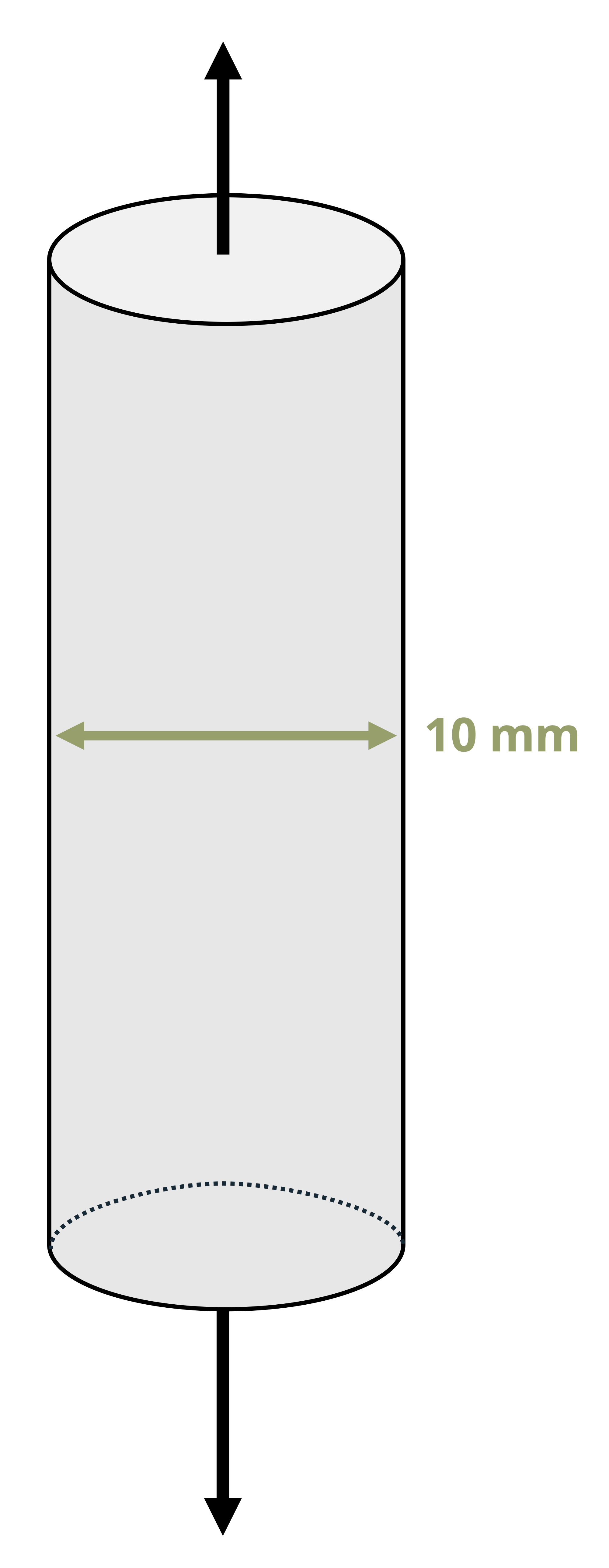
A circular polymeric rod with a diameter of 10 mm is subjected to a uniaxial force, resulting in an axial strain of 0.5%. A corresponding reduction in diameter of 0.02 mm is measured. Determine the Poisson’s ratio of this material.
4.5 Shear Stress/Strain
Click to expand
In addition to considering normal stresses and strains, an understanding of the relationship between shear stresses and shear strains is also needed. A similar experiment can be performed to produce a diagram of shear stress against shear strain. The slope of a shear stress versus shear strain diagram is referred to as the shear modulus or modulus of rigidity, and will be designated by G. The corresponding slope of a shear stress versus shear strain plot is referred to as the shear modulus or modulus of rigidity, as shown in Figure 4.6 (B).
\[ \boxed{\tau=G \gamma} \tag{4.3}\]
𝜏 = Shear stress [Pa, psi]
G = Shear modulus or modulus of rigidity [Pa, psi]
𝛾 = shear strain
It should be noted that Young’s modulus, the shear modulus, and Poisson’s ratio are not all independent of one another. For isotropic materials, there are only two independent, linear elastic properties; knowing any two allows one to calculate the others. It can be shown that:
\[ \boxed{G=\frac{E}{2(1+v)}} \tag{4.4}\]
G = Shear modulus or modulus of rigidity [Pa, psi]
E = Elastic modulus [Pa, psi]
𝜈 = Poisson’s ratio
See Example 4.3 for a problem involving the shear modulus.
Example 4.3
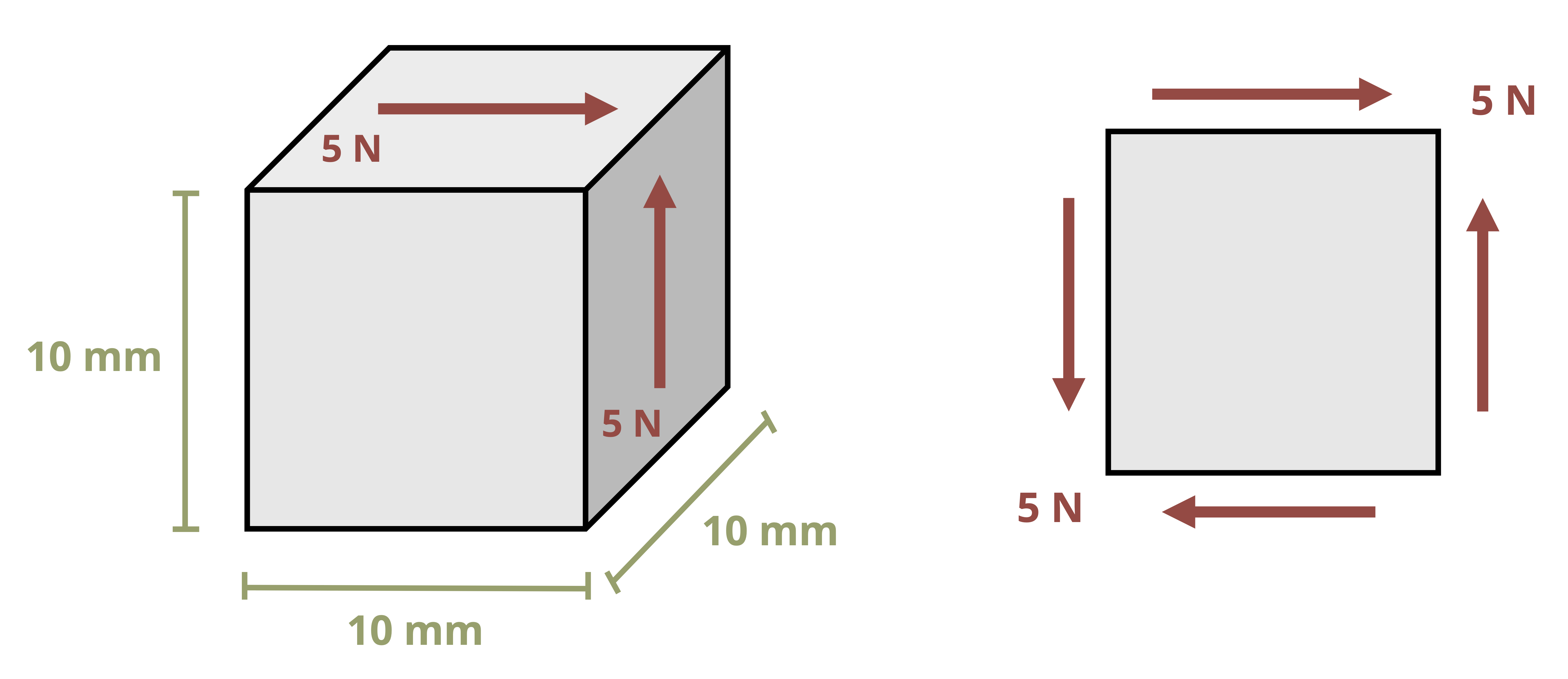
Soft contact lenses often consist of a hydrogel, an elastomeric network that is imbibed with water, expanding its volume and making the lens more soft and compliant. Suppose a 10 mm cube of the dry elastomer were subjected to a shearing action as shown. Shearing forces of 5 N each are applied to the four faces of the cube, resulting in a displacement of 0.3 mm. What is the shear modulus of this elastomeric block?
4.6 Thermal Strain
Click to expand
In addition to relationships arising between stress and strain, other factors can affect dimensional changes of materials as well as changes in the stresses present in a structure. Most materials will expand, for example, when their temperature is increased. Many engineering structures will experience significant temperature variations during their life, beginning with thermal processes involved in their manufacture, cyclic temperature changes (e.g., day/night or summer/winter), or because of their usage, such as an engine block heating up or cooling down. Though dimensional changes from temperature often appear to be quite small, they can lead to significant changes in stress state, and in fact numerous failures result not from applied mechanical loading but from thermal exposure issues. Though beyond the current scope, other dimensional changes can also result from other environmental factors, such as the expansion of a material as water is absorbed, or from the application of electric fields for materials that exhibit piezoelectric properties.
Vibrational energy of atoms increases as temperature increases, typically leading to slightly greater atomic separation distances. This expansion leads to dimensional changes in the material, and the behavior is characterized by the material’s coefficient of thermal expansion (CTE). The linear CTE is often designated by \(\alpha\) and is defined as the change in strain per unit change in temperature. As with the other material properties discussed in this chapter, \(\alpha\) is assumed to be constant for any given material.
The CTE is independent of direction in isotropic materials. One may determine the CTE by heating or cooling a specimen and measuring the resulting strain (ε) or dimensional change and recording the change in temperature (ΔT):
\[ \alpha=\frac{\varepsilon}{\Delta T}=\frac{\frac{\Delta L}{L}}{\Delta T} \]
where \(\Delta T=T_{final}-T_{initial}\). Since strain is unitless, CTE has units of \(\frac{1}{{ }^{\circ} \mathrm{C}}\) or \(\frac{1}{{ }^{\circ} F}\). Knowing the CTE, one can easily determine the strain expected when a material is subjected to a temperature change of ΔT:
\[ \boxed{\varepsilon_T=\alpha \cdot \Delta T} \tag{4.5}\]
Or dimensional changes can be determined as:
\[ \boxed{\Delta L=\alpha \cdot \Delta T \cdot L} \tag{4.6}\]
𝜀T = Thermal strain
𝛼 = Coefficient of thermal expansion \(\left[\frac{1}{^\circ C},\frac{1}{^\circ F}\right]\)
𝛥T = Change in temperature \([^\circ C, ^\circ F]\)
𝛥L = Change in length [m, in.]
L = Original length [m, in.]
See Example 4.4 for a problem involving a temperature change resulting in a thermal strain.
Example 4.4
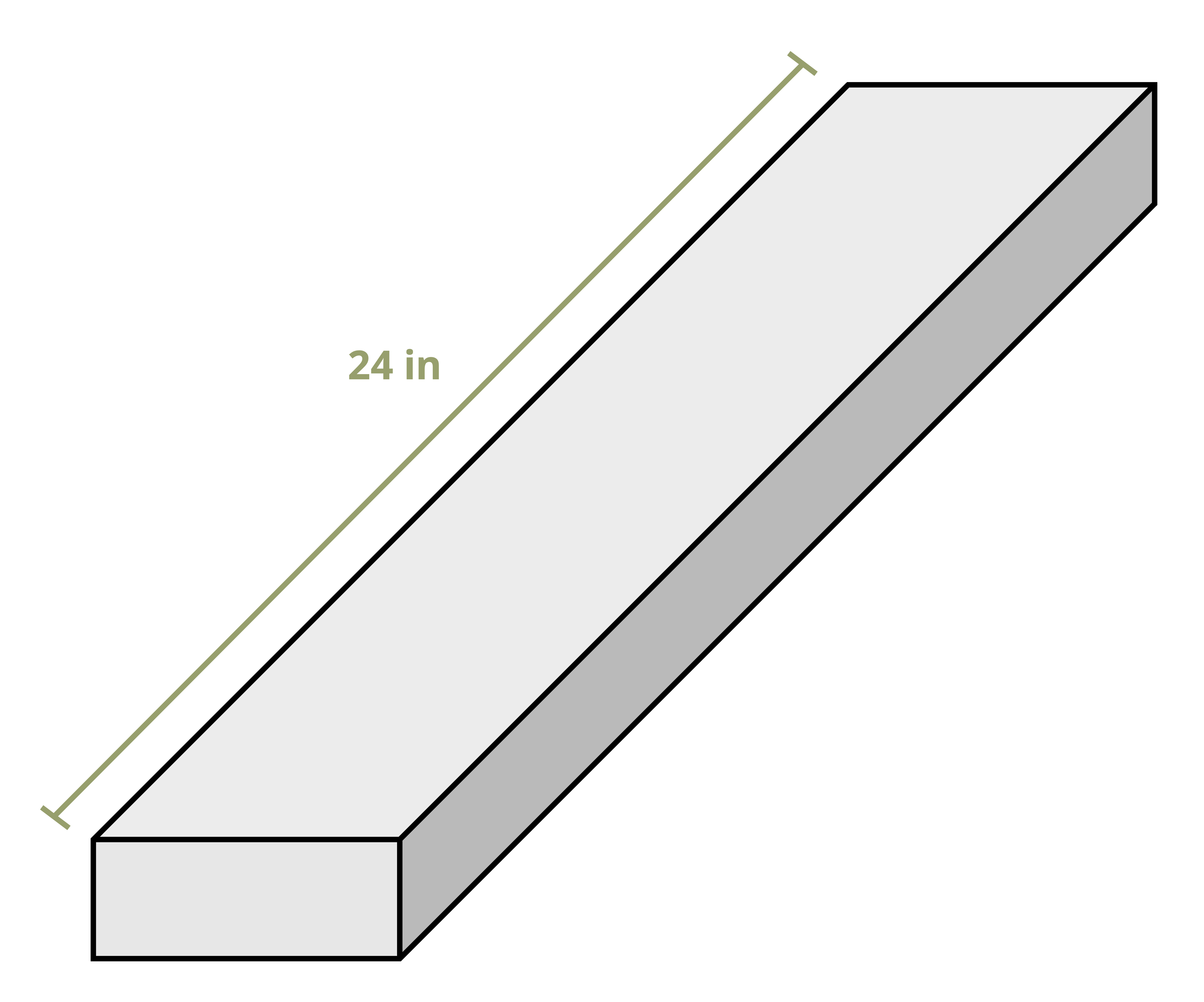
A 24” long aluminum bar with a coefficient of thermal expansion of 13x10-6/F° and Young’s modulus of 10,000 ksi is cooled from 100°F to 25 °F.
- What change in strain results from this temperature change if the bar is free to contract?
- What change in length results from this temperature change if the bar is free to contract?
4.7 Multiaxial or Generalized Hooke’s Law
Click to expand
Materials are often tested under idealized conditions, such as uniaxial tension or shearing resulting from torsional loading. These tests are important because they provide material properties necessary for engineering design. Such simple stress states are less common in actual engineered components, where more complex, multiaxial stress states are present, as shown in Figure 4.7.
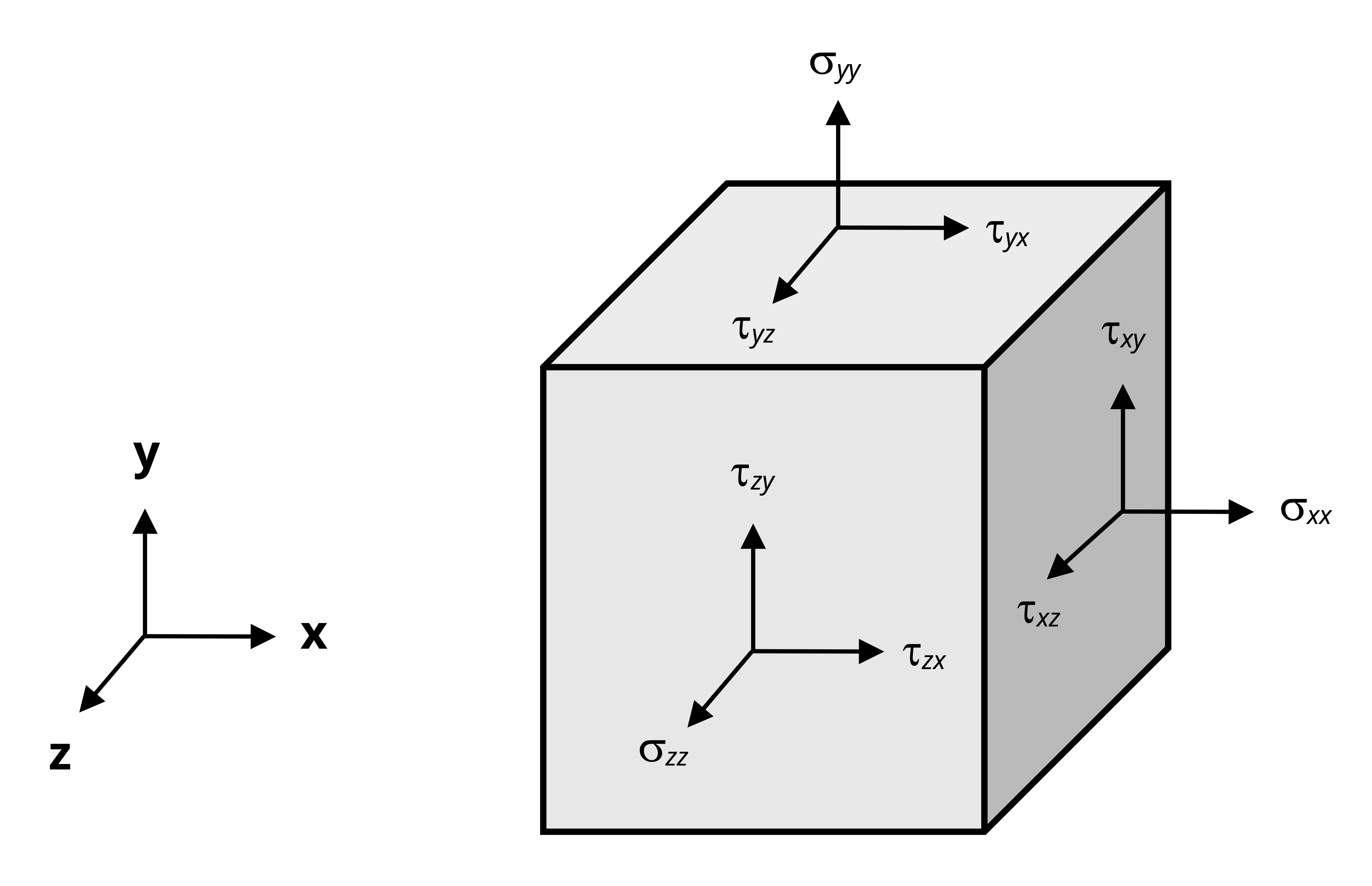
Here there are three normal stresses, referred to with a single subscript indicating their direction (σx, σy, and σz). There are six shear stresses, designated by τ, which are referred to with two subscripts, one indicating the plane or ‘face’ that the stress acts on and the other indicating the direction that it acts in. For example, on the y-z plane (the x-face) there is the normal stress σx and two shear stresses, τxy and τxz. The first subscript indicates that these shear stresses act on the x-face and the second subscript indicates that they point in the y- and z-directions respectively.
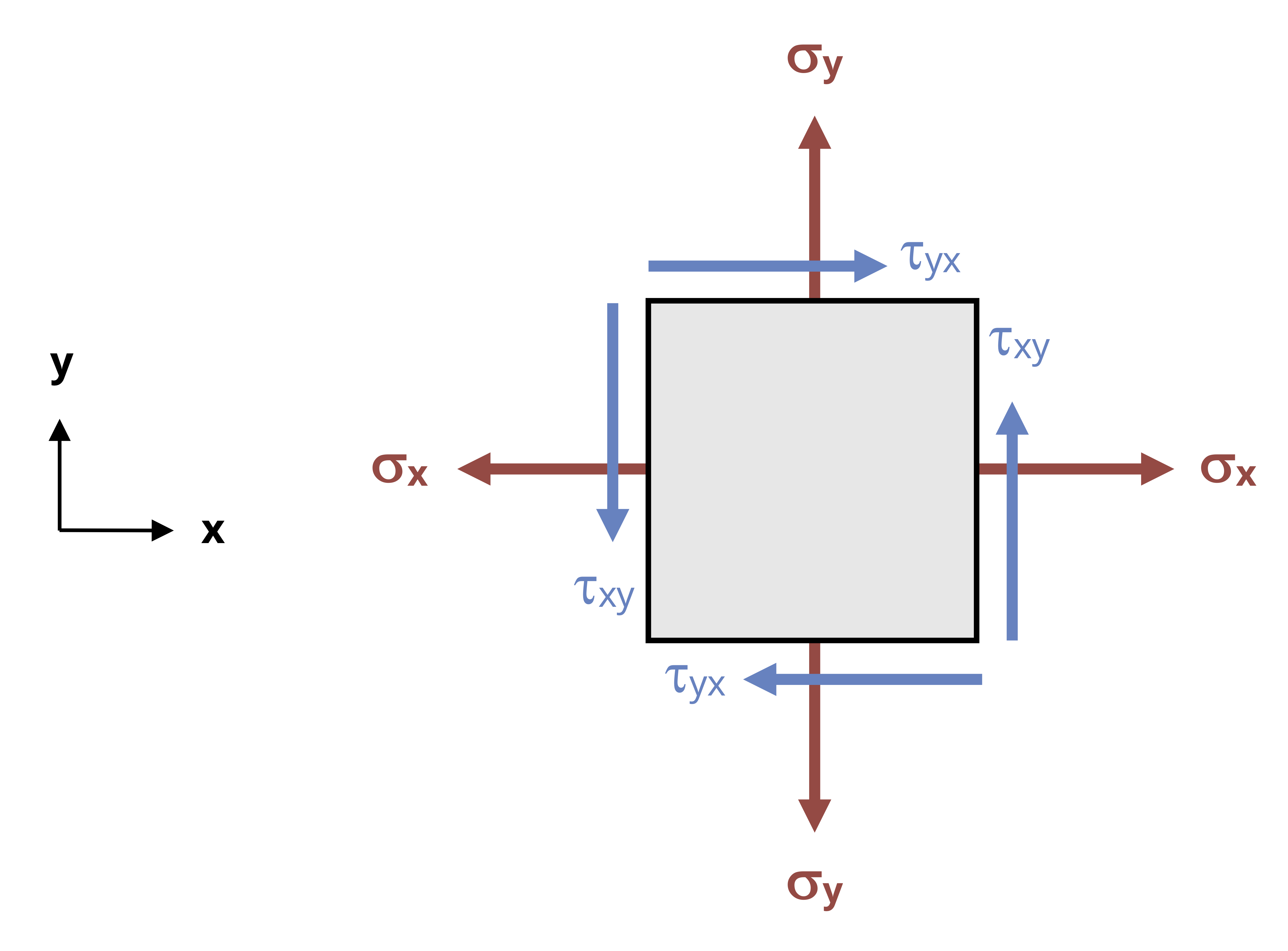
Consider the x-y plane of the stress element in Figure 4.7. This 2D plane is shown in Figure 4.8. It experiences two normal stresses (σx and σy) and two shear stresses (τxy and τyx). τxy will cause the element to rotate counterclockwise while τyx will cause the element to rotate clockwise. For an element in equilibrium, these two stresses must be equal in order for these rotation effects to balance. Expanding this to the other planes we may say τxy = τyx, τxz = τzx, and τyz = τzy.
Having learned the concept of Poisson’s ratio, we recognize that there is a coupling between normal stresses in one direction and the normal strains in other directions. We have reviewed this in the context of the response to the application of a uniaxial stress state—a normal stress applied in only one direction. For example, if there is a normal stress in the x-direction there will also be a normal strain in the x-direction and also in the y- and z-directions.
Specifically:
\[ \begin{aligned} & \varepsilon_x=\frac{\sigma_x}{E} \\ & \varepsilon_y=-v \varepsilon_x=-\frac{\nu \sigma_x}{E} \\ & \varepsilon_z=-\nu \varepsilon_x=-\frac{\nu \sigma_x}{E} \end{aligned} \]
Most engineering structures, however, involve more complex stress states, in which stresses may be applied in the x-, y-, and z-directions. We refer to these as multiaxial stress states. We can define similar equations for a normal stress applied in the y-direction:
\[ \begin{aligned} & \varepsilon_y=\frac{\sigma_y}{E} \\ & \varepsilon_x=-\nu \varepsilon_y=-\frac{\nu \sigma_y}{E} \\ & \varepsilon_z=-\nu \varepsilon_y=-\frac{\nu \sigma_y}{E} \end{aligned} \]
And for a normal stress applied in the z-direction:
\[ \begin{aligned} & \varepsilon_z=\frac{\sigma_z}{E} \\ & \varepsilon_x=-\nu \varepsilon_z=-\frac{\nu \sigma_z}{E} \\ & \varepsilon_y=-\nu \varepsilon_z=-\frac{\nu \sigma_z}{E} \end{aligned} \]
If loads are applied in all 3 directions simultaneously, we can determine the overall strain in each direction by simply adding together the above components:
\[ \boxed{\begin{aligned} & \varepsilon_x=\frac{\sigma_x}{E}-\frac{\nu \sigma_y}{E}-\frac{\nu \sigma_z}{E}=\frac{1}{E}\left[\sigma_x-\nu\left(\sigma_y+\sigma_z\right)\right] \\ & \varepsilon_y=\frac{1}{E}\left[\sigma_y-\nu\left(\sigma_x+\sigma_z\right)\right] \\ & \varepsilon_z=\frac{1}{E}\left[\sigma_z-\nu\left(\sigma_x+\sigma_y\right)\right] \end{aligned}} \tag{4.7}\]
𝜀x, 𝜀y, 𝜀z = Normal strain in the x-, y-, and z-directions
𝜎x, 𝜎y, 𝜎z = Normal stress in the x-, y-, and z-directions [Pa, psi]
E = Elastic modulus [Pa, psi]
𝜈 = Poisson’s ratio
This is the generalized Hooke’s law for the 3-dimensional state of stress. Example 4.5 demonstrates the application of the generalized Hooke’s law to a problem with stresses acting in the x-, y-, and z-directions.
We may make similar observations about strain, where normal strains are written with a single subscript as εx, εy, and εz. Shear strains are written with 2 subscripts as γxy = γyx, γxz = γzx, and γyz = γzy.
The relationships between shear stresses and strains do not change in isotropic materials subjected to additional other stress components, so:
\[ \boxed{\begin{aligned} & \gamma_{xy}=\frac{\tau_{xy}}{G} \\ & \gamma_{yz}=\frac{\tau_{yz}}{G} \\ & \gamma_{xz}=\frac{\tau_{xz}}{G} \end{aligned}} \tag{4.8}\]
𝛾xy, 𝛾yz, 𝛾xz = Shear strains
𝜏xy, 𝜏yz, 𝜏xz = Shear stresses [Pa, psi]
G = Shear modulus [Pa, psi]
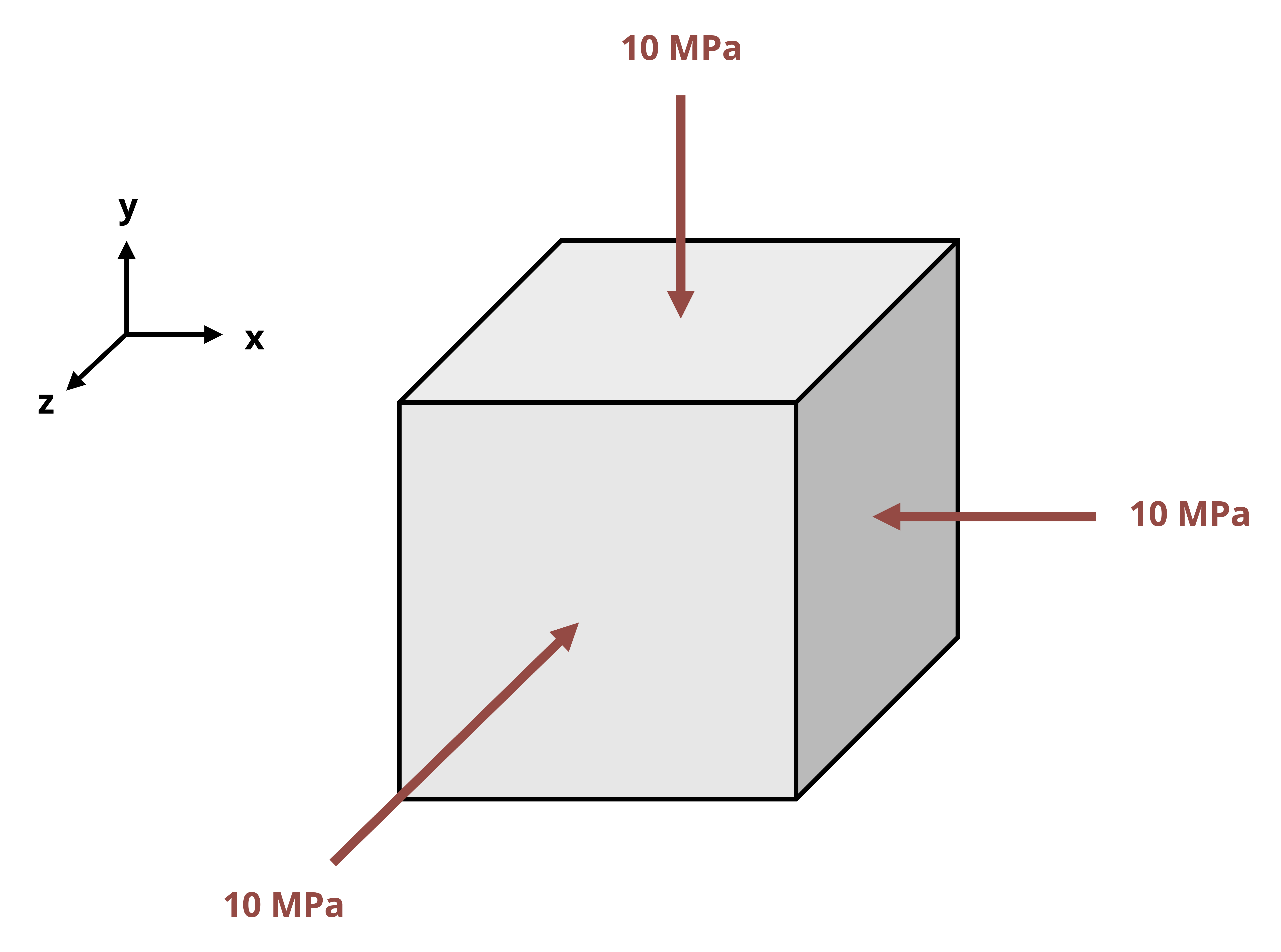
Example 4.5
A solid, 50 mm polycarbonate cube is subjected to a compressive stress of \(p=10 \mathrm{MPa}\) on all sides. Assuming the material has a Young’s modulus of 3 GPa and a Poisson’s ratio of 0.38, what is the change in length of one of the edges?
4.8 Allowable Stress/Safety Factor
Click to expand
Safety is of primary importance in engineering practice, and various engineering principles and codes are built on the necessity of considering the safety of products we design. The concept is that we would determine the location and magnitude of the maximum stresses under the most stringent anticipated loading conditions and compare these predicted values with the failure stress, such as the yield or ultimate strength of a material. Rather than allowing the maximum anticipated stress to equal the failure stress, however, products are often designed so that the maximum allowable stress is only some fraction of the failure stress, leading to a more conservative design. Essentially, the failure stress is scaled back by the factor of safety (F.S.), a quantity that is greater than one.
\[ \boxed{\sigma_{allow}=\frac{\sigma_{fail}}{F . S .}} \tag{4.9}\]
𝜎allow = Allowable stress [Pa, psi]
𝜎fail = Failure stress [Pa, psi]
F.S. = Factor of safety
Example problem 4.6 demonstrates a simple calculation of the factor of safety based on the failure and allowable stresses in a component. In practice it is also common to work the other way and, starting with a defined factor of safety and failure stress, calculate the allowable stress in a component made of a given material.
Making the factor of safety larger, in principle, should make the structure less likely to fail, but there are often weight, cost, environmental, and functional penalties associated with higher F.S. values. If the F.S. value is too small, the margin of safety for the design may become unacceptable. Unexpected overload situations, engineering design and assumption errors, and general wear and tear of a material over time, including in challenging environments, could lead to failure. The consequences of failures can range from minor inconveniences all the way to major catastrophes with significant loss of life and property. Negative publicity and attitudes towards even minor failures can be of concern to customers and significantly reduce future product sales, so product engineering involves risk assessment and mitigation, in addition to production costs and other factors.
Safe design philosophies are often industry-specific and may be much more involved and complicated than our simple factor of safety concept conveys. For our purposes, suffice it to say that larger factors of safety are often used when there is less certainty about our designs, the loads our structures might sustain, or the severity of environmental and use conditions. Larger factors of safety are often required when the consequences of failure are considered to be greater. For example, design of a theatre that could be filled with hundreds of people might use a higher F.S. than that employed for a storage building that is seldom occupied. Example 4.6 demonstrates the use of factor of safety in a design.
Example 4.6
A 2 mm diameter steel wire is used to suspend a mass of 40 kg. Using the yield strength of 200 MPa as the allowable stress, what is the factor of safety of the wire (ignoring end and dynamic effects)?