12 Stress Transformation
Introduction
Click to expand
In Section 4.7 we discussed the general state of stress. Figure 4.7 shows a 3D stress element subjected to the general state of stress – that is, 3 normal stresses (σx, σy, and σz) and 6 shear stresses τxy, τxz, τyx and τyz, τzx and τzy.
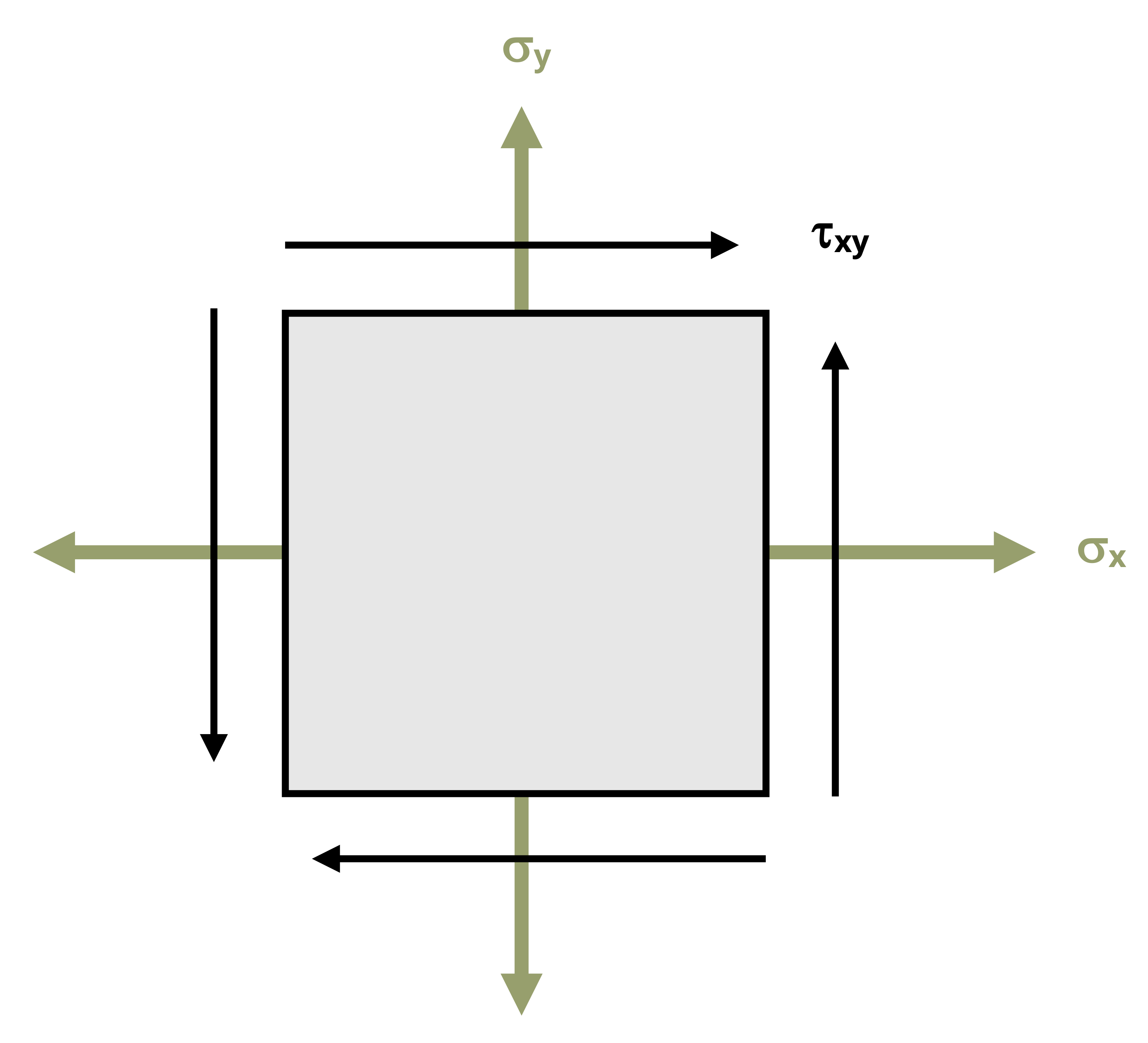
Figure 4.8 shows a stress element for the simplified case of plane stress – that is, stresses acting in a single plane. Under plane stress, the element experiences normal stresses σx and σy, and shear stress τxy = τxz.
These stress elements are a convenient way to show the stresses at a particular orientation of the stress element, often in the x-y plane. However, we sometimes want to know the stresses at different orientations. For example, in Section 2.4 we learned how to calculate the stresses on inclined planes. There we were calculating the stresses at specific orientations that were not in the x-y directions, but rather at some angle relative to the x-y directions.
In this chapter we will develop a more general approach where we can begin with the stresses in any given direction (usually starting with the x-y directions is simplest) and use these stresses to calculate the stresses at different orientations of the stress element. This process is known as stress transformation.
In Section 12.1 we will develop equations that allow us to begin with normal and shear stresses in the x-y directions and transform them to determine the stresses at any other orientation.
In Section 12.2 we will expand on these equations in order to determine the maximum and minimum stresses, as well as the orientations that they occur at.
In Section 12.3 we will discuss an alternative graphical method for performing stress transformation, known as Mohr’s circle.
In Section 12.4 we will use Mohr’s circle to expand our analysis and look at the stresses not only in the original 2D plane, but also at the out-of-plane stresses.
12.1 Stress Transformations
Click to expand
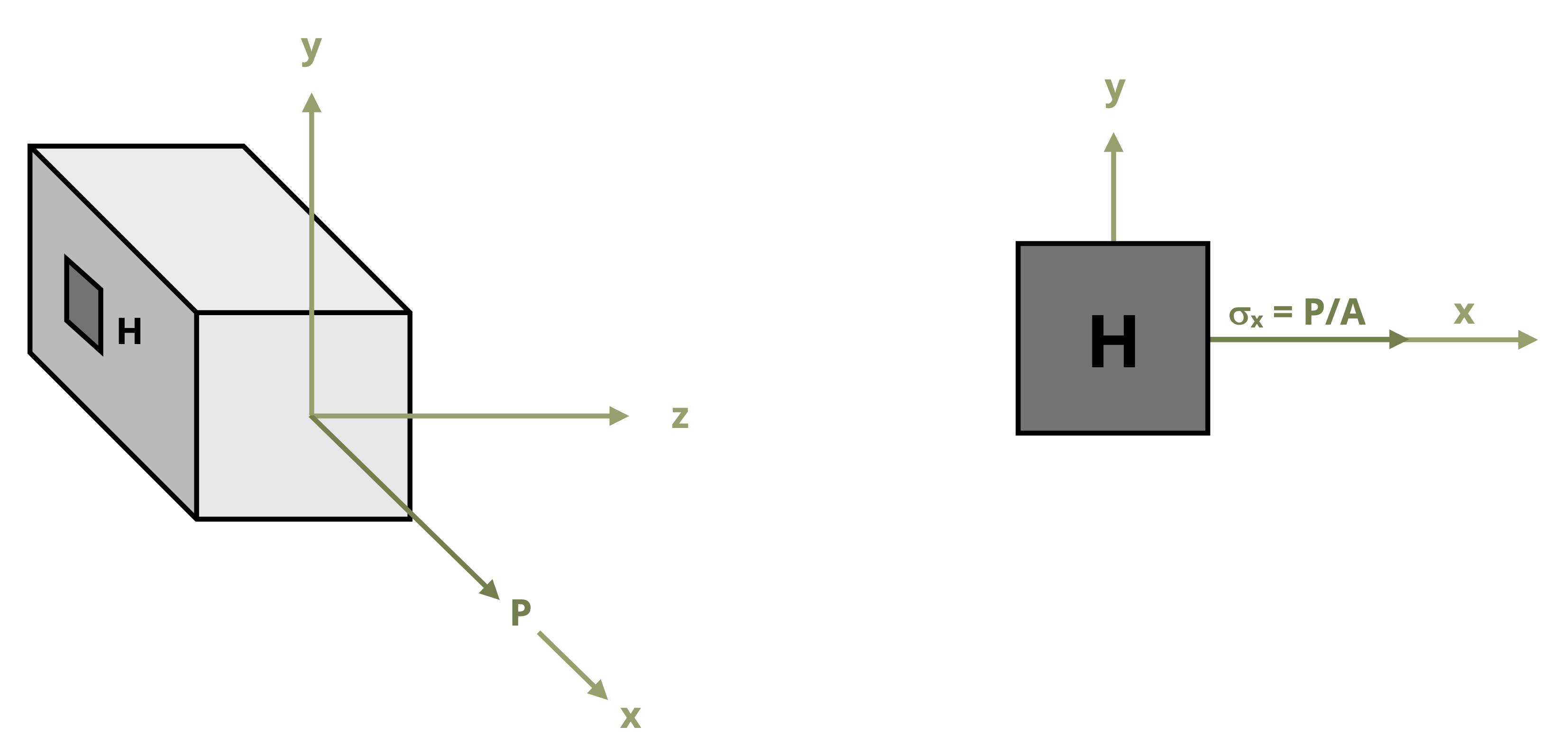
The choice of a coordinate system to use when calculating stresses for a given loading condition is often chosen based on convenience, or what is considered to be the most straight forward system for the given loading directions and the geometrical orientation of the body. For example, consider the simple case of an axial load applied to a rectangular bar as shown in Figure 12.1. It is convenient to use a coordinate system in which one axis aligns with the longitudinal axis of the bar and the other two axis aligned with the edges of the cross-section. With this coordinate system, the general stress state can be quickly determined to consist of only a normal stress in the x direction. We can represent the state of stress at a given point, say point H, on a stress element. Remember that this stress element is actually a 3D object even though we typically draw a 2D plane view of the element.
However, the coordinate systems that are the most straightforward to base stress calculations on do not always represent the directions for which the stress levels are the most critical. In the above example, if the bar consists of two sections glued together at an angle, or if the bar is made of wood or composite material with the grains or fibers running at angle to the horizontal, one might be concerned with the level of stress parallel and/or perpendicular to the joint surface (or grains/fibers).
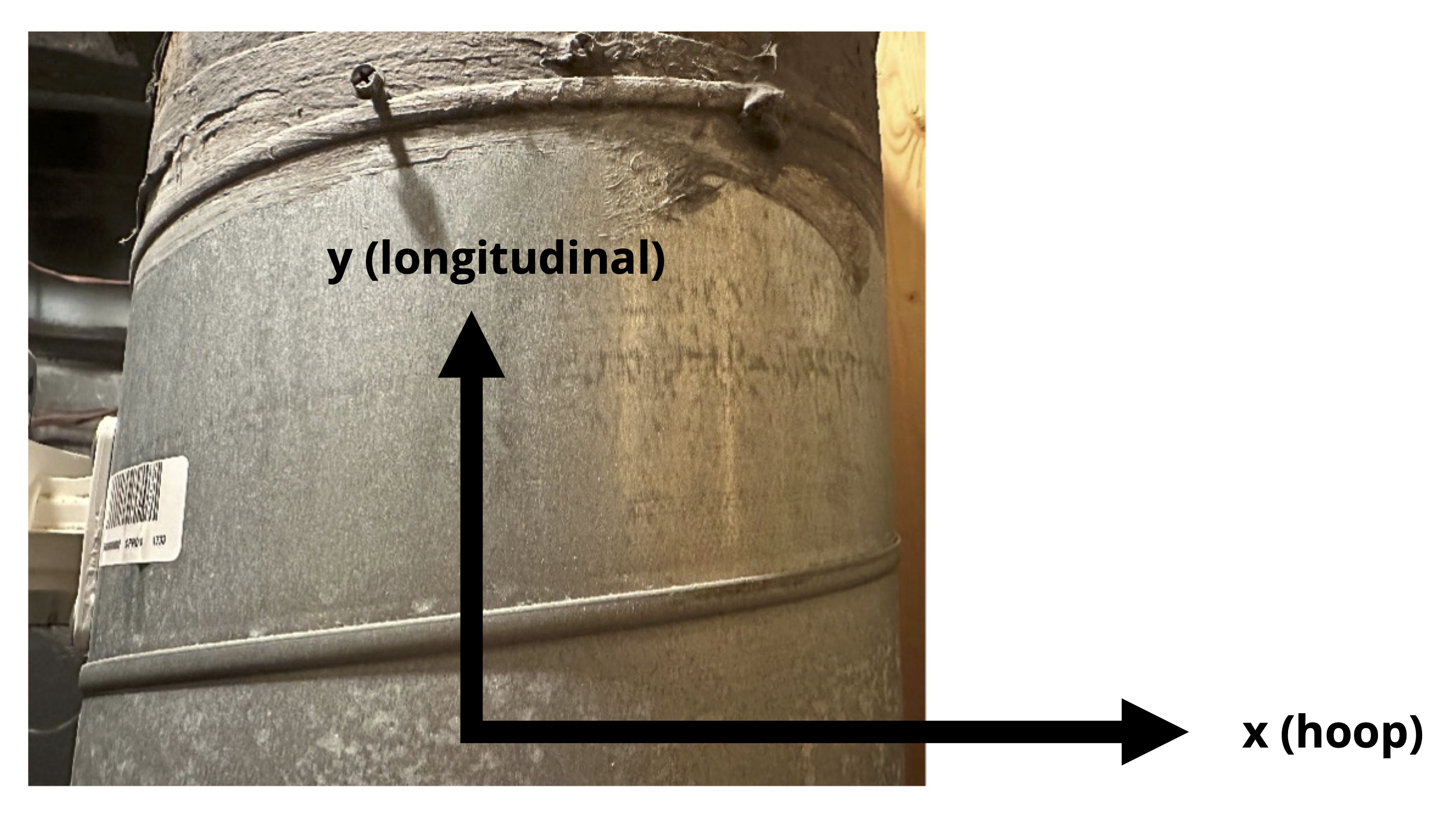
Figure 12.2 shows an air duct which is part of a heat pump system and is subject to internal air pressure. Pressure vessels will be discussed in Chapter 13 and it will be shown that equations to calculate stress based on pressure and geometrical parameters in the longitudinal and hoop directions can be straightforwardly derived. However, as is the case for the duct in the figure, pressure vessels can often be made with welded seams wound in a helical pattern that forms an angle with the horizontal and vertical axes. It would be important to know the stresses in the directions parallel and perpendicular to these seams to ensure that the joint could tolerate the loading.
Now we’ll use trigonometry to develop a general set of equations to transform stresses from one set of coordinate axes to another. Consider a stress element representing the state of stress at a point in the xy plane as shown in Figure 12.3. If we want to use the known stresses in the xy coordinate system to find the stresses parallel and perpendicular to a different plane, represented by the incline shown on the element, we can cut through the element at the appropriate angle and consider the free body diagram on the cut section. The FBD of the cut element shows the known stresses on the uncut sides of the element and the unknown internal reaction normal and shear stresses, σn and τnt, on the cut side of the element. The internal reactions are represented in the directions for which we want to know the stress state.
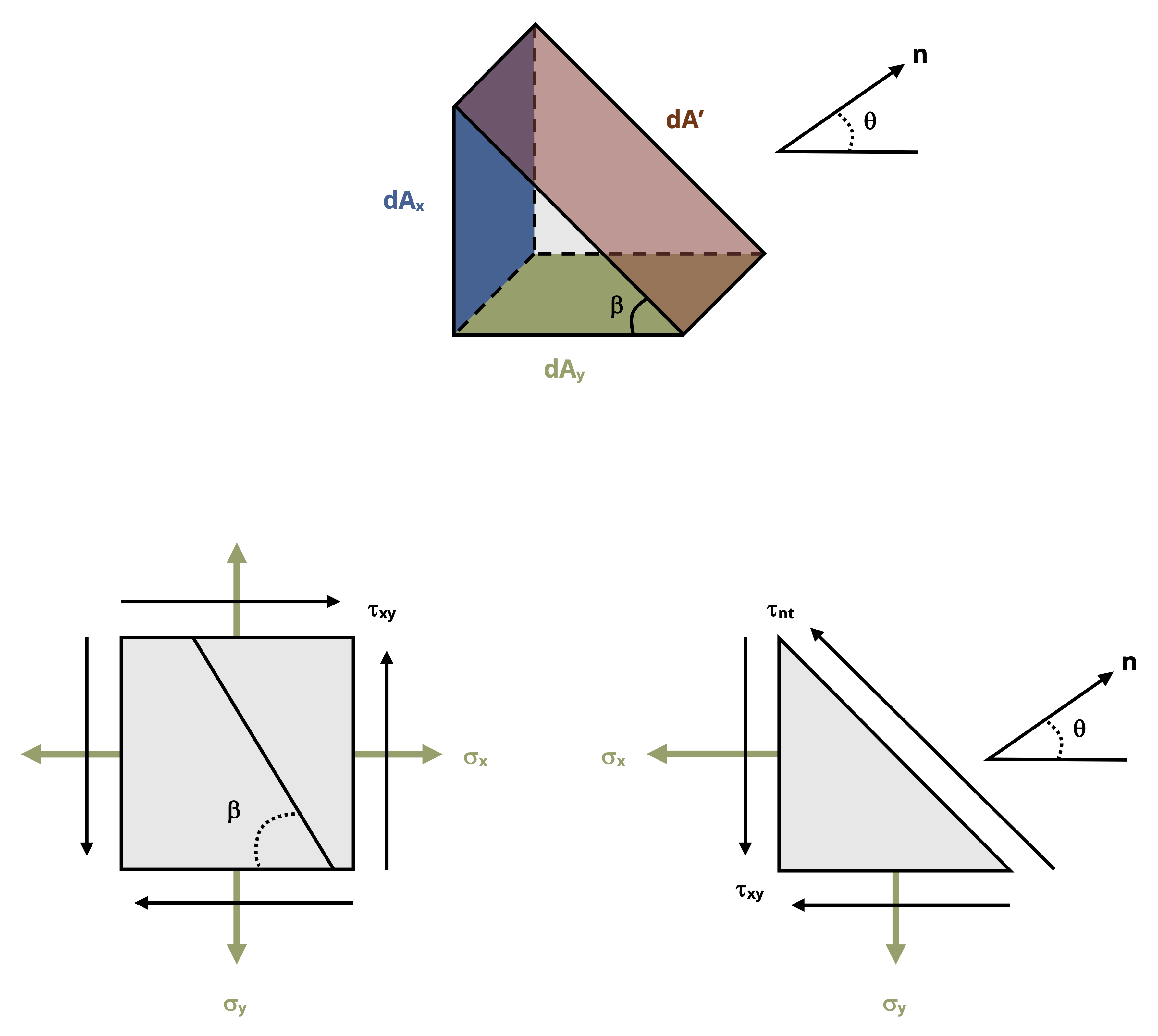
Consider the area of the cut side of the element on which σn and τnt act to be dA’. By applying trigonometry we can say that the area of the side on which σx acts, dAx, is:
\[ d A_x=d A^{\prime}(\sin \beta)=d A^{\prime} \cos (\theta) \]
and the area of the side on which σy acts is:
\[ d A_x=d A^{\prime}(\cos \beta)=d A^{\prime} \sin (\theta) \]
We can apply equilibrium to obtain expressions for σn and τnt if we express the stress components as forces and resolve those forces into the n and t directions. The force corresponding to each direction of stress is obtained by multiplying the stress with the area it acts on (i.e., the force corresponding to σx is σx*dAx).
From σx we have:
\[ \begin{aligned} & F_n=-\sigma x^* d A x^* \cos (\theta)=-\sigma x^* d A^{\prime} \cos (\theta) \cos (\theta) \\ & \mathrm{Ft}=\sigma x^* \mathrm{~d} A x^* \sin (\theta)=\sigma x^* d A^{\prime} \cos (\theta) \sin (\theta) \end{aligned} \]
From σy we have:
\[ \begin{aligned} & F_n=-\sigma y^* d A y^* \sin (\theta)=-\sigma y^* d A^{\prime} \sin (\theta) \sin (\theta) \\ & F t=-\sigma y^* d A y^* \cos (\theta)=-\sigma y^* d A^{\prime} \cos (\theta) \sin (\theta) \end{aligned} \]
From the vertical shear stress acting on the x-face we have:
\[ \begin{aligned} & F n=-\tau_{xy}{ }^* d A x^* \sin (\theta)=-\tau x y^* d A^{\prime} \cos (\theta) \sin (\theta) \\ & F t=-\tau_{xy}{ }^* d A x^* \cos (\theta)=-\tau x y^* d A^{\prime} \cos (\theta) \cos (\theta) \end{aligned} \]
From the horizontal shear stress acting on the y face we have:
\[ \begin{aligned} & \mathrm{Fn}=-\tau_{xy} *^* d A x^* \cos (\theta)=-\tau x y^* d^{\prime} \sin (\theta) \cos (\theta) \\ & F t=\tau_{xy}{ }^* d A y^* \sin (\theta)=\tau_{x y}^* d A^{\prime} \sin (\theta) \sin (\theta) \end{aligned} \]
Applying equilibrium in the n and t directions:
\[ \begin{gathered} \sum F_n=-\sigma_x * d A^{\prime} * \cos ^2(\theta)-\sigma_y * d A^{\prime} * \sin ^2(\theta)-2 \tau_{x y} * d A^{\prime} * \cos (\theta) \sin (\theta)=0 \\ \sum F_t=\sigma_x * d A^{\prime} * \cos (\theta) \sin (\theta)-\sigma_y * d A^{\prime} * \cos (\theta) \sin (\theta)+\tau_{x y} * d A^{\prime} *\left(\sin ^2(\theta)-\cos ^2(\theta)\right) \\ +\tau_{n t} d A^{\prime}=0 \end{gathered} \]
Solving the equations for σn and τnt and simplifying terms gives:
\[ \begin{aligned} & \sigma_n=\sigma_x \cos ^2(\theta)+\sigma_y \sin ^2(\theta)+2 \tau_{x y} \sin (\theta) \cos (\theta) \\ & \tau_{n t}=-\left(\sigma_x-\sigma_y\right) \cos (\theta) \sin (\theta)+\tau_{x y}\left(\cos ^2(\theta)-\sin ^2(\theta)\right) \end{aligned} \]
These equations are known as the stress transformation equations.
Alternatively, implementing the trig identities:
\[ \begin{gathered} \cos ^2(\theta)=\frac{1+\cos (2 \theta)}{2} \\ \sin ^2(\theta)=\frac{1-\cos (2 \theta)}{2} \\ \sin (2 \theta)=2 \sin (\theta) \cos (\theta) \\ \cos (2 \theta)=\cos ^2(\theta)-\sin ^2(\theta) \end{gathered} \]
The transformation equations can also be expressed as:
\[ \boxed{\begin{aligned} \sigma_n & =\frac{\sigma_x+\sigma_y}{2}+\frac{\sigma_x-\sigma_y}{2} \cos (2 \theta)+\tau_{x y} \sin (2 \theta) \\ \tau_{n t} & =-\frac{\sigma_x-\sigma_y}{2} \sin (2 \theta)+\tau_{x y} \cos (2 \theta) \end{aligned}} \tag{12.1}\]
𝜎n = Average normal stress perpendicular to the inclined plane [Pa, psi]
𝜏nt = Average shear stress parallel to the inclined plane [Pa, psi]
𝜎x = Average normal stress in the x-direction, prior to any transformation [Pa, psi]
𝜎y = Average normal stress in the y-direction, prior to any transformation [Pa, psi]
𝜏xy = Average shear stress in the xy plane, prior to any transformation [Pa, psi]
𝜃 = Angle between x-axis and transformed stress being caculated [\(^\circ\), rad]
Either set of transformation equations will work. The choice over which set to use is based on personal preference.
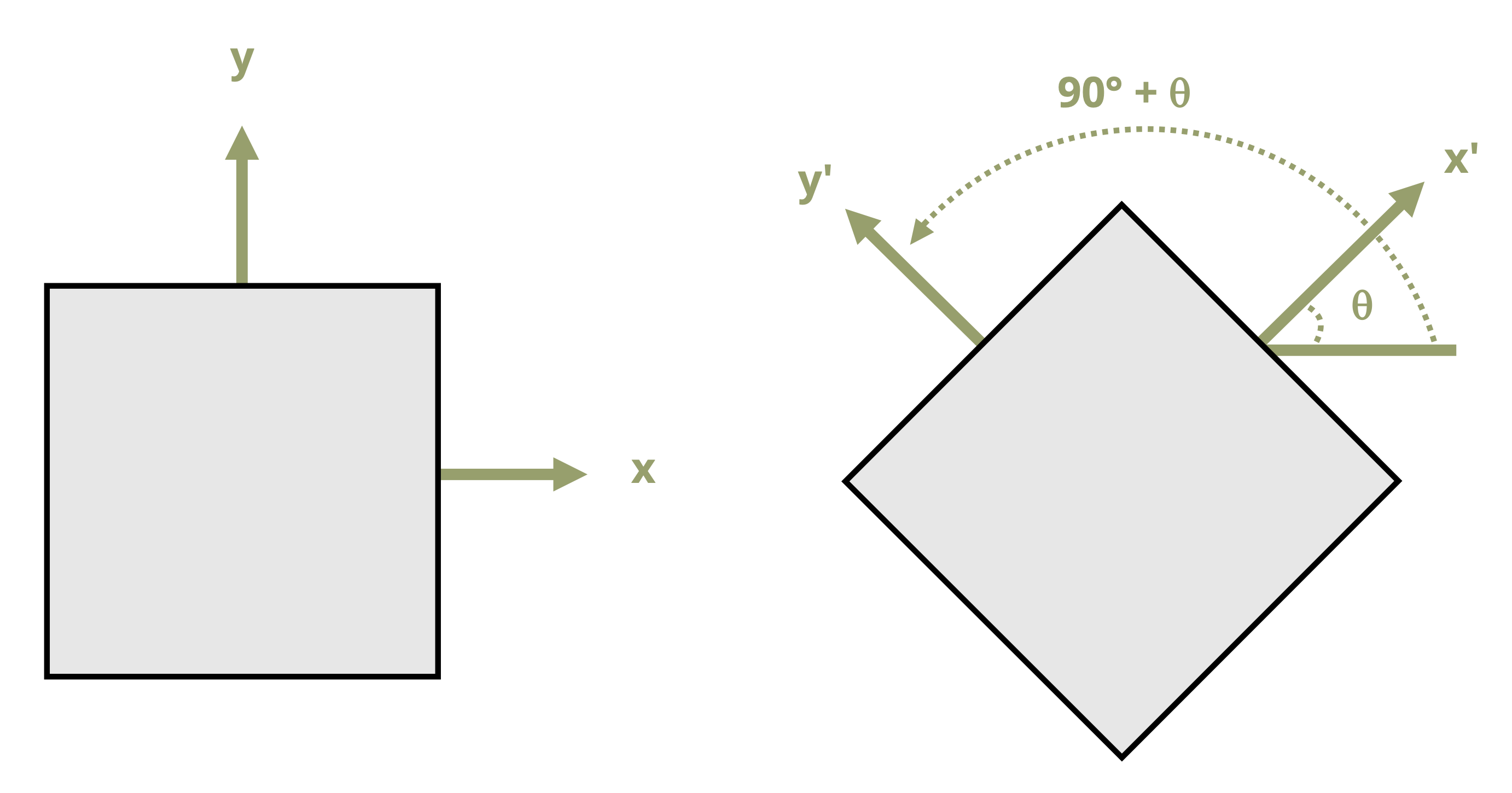
The stress transformation equations can be used to take a set of stresses calculated in the chosen coordinate system (xy) and transform them to a different coordinate system (x’y’), as shown in Figure 12.4. With θ defined to be the angle between the x-axis and the normal to the plane of interest as shown in Figure 12.3, the σn equation gives the stress on the rotated x-face, which we will call the σx’. To find σy’, the normal stress on the rotated y-face, we can simply sub an angle of (90° + θ) into the σn equation since the y’ axis would be rotated an additional 90° form the x-axis. Also note that substituting θ into the τnt equation gives τx’y’.
Another way to quickly determine the normal stress along the y’ axis once σx’ is known is to make use of the concept of stress invariance which is the idea that sum of the normal stresses (σx + σy) remains constant regardless of the plane in which they are calculated. Put another way, the stress invariance principle allows us to say that (σx + σy) = (σx’ + σy’).
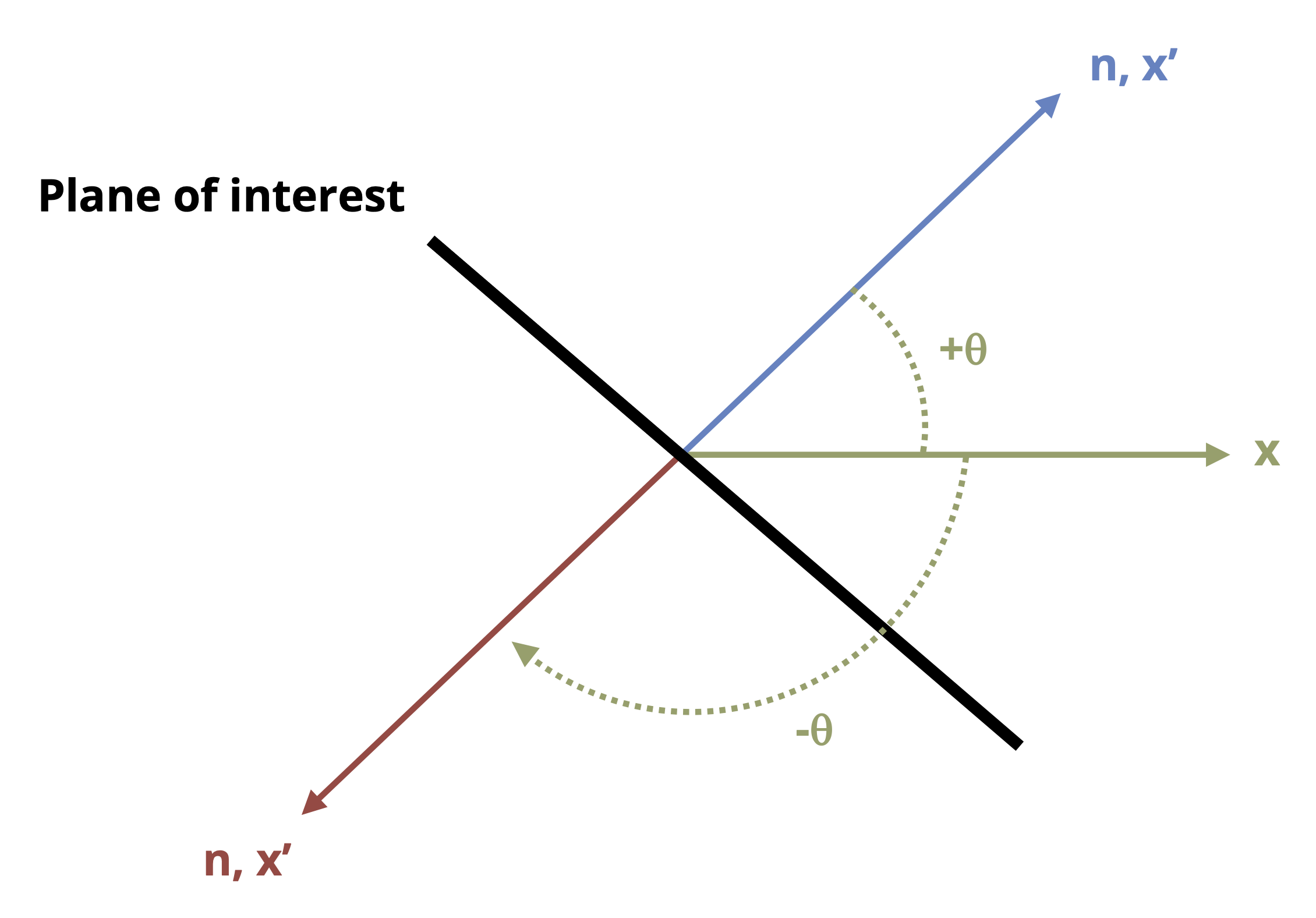
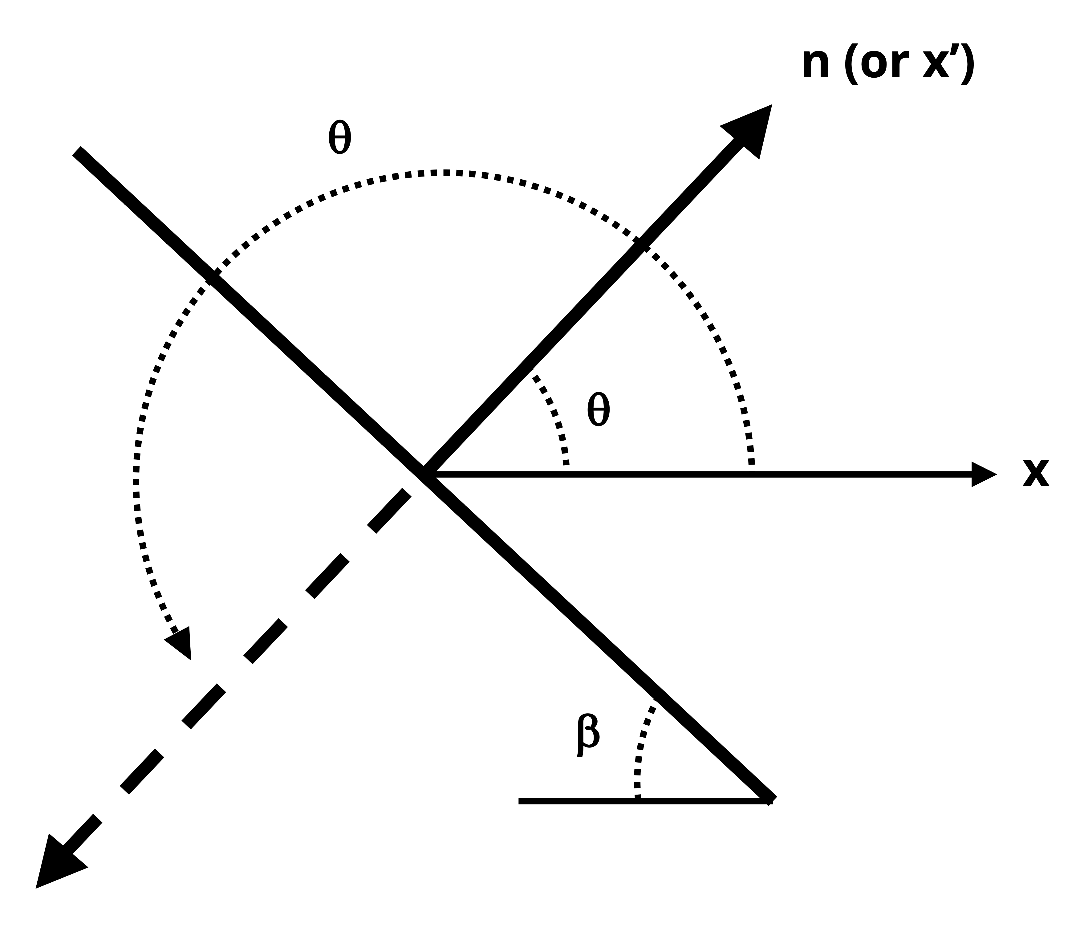
The angle of incline may be measured and given relative to a variety of reference axes. It is imperative that one understands which angle to substitute into the transformation equations given above. To ensure you have the correct angle, take the following steps and see Figure 12.5:
Draw a line that represents the plane of interest
Draw the x-axis positive going towards the right
Draw the axis normal to the plane of interest. It does not matter if you draw the normal axis as oriented counterclockwise or clockwise from the x-axis as long as you use the correct sign for the angle (see step 4).
Determine the angle that goes from the x-axis to the normal axis. This angle is θ. If the direction from the x-axis to the normal axis is counterclockwise, then θ should be taken to be positive. If the direction from the x-axis to the normal axis is clockwise, then θ should be taken to be negative.
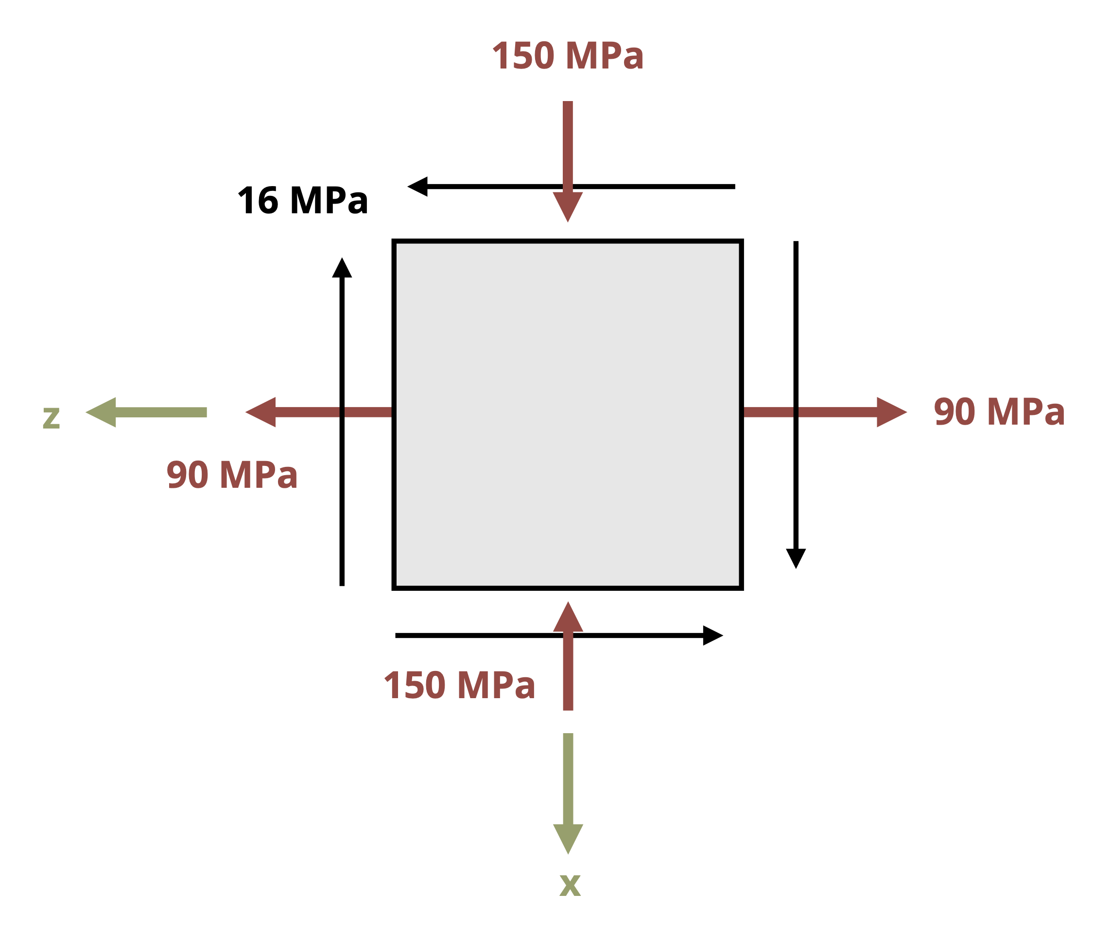
Finally, one should note that the transformation equations were derived based on stresses given in the the x-y plane where x is the horizontal axis positive to the right and y is the vertical axis positive upwards. If a plane other than the xy plane is being used for the general stress calculations, or if the x and y axes are oriented in the opposite configuration, the rule to follow would be to substitute the stress normal to the vertical faces of the element in for the σx terms of the equations and the stress normal to the horizontal faces of the element in the σy terms of the equations. For example, given the stress element in Figure 12.6, one would substitute σz = 90 MPa in for the σx terms of the stress transformation equations, σx = -150 MPa in for the σy terms, and τxz = -16 MPa in for the τxy terms.
Example 12.1 and Example 12.2 below illustrate the use of the stress of transformation equations.
Example 12.1
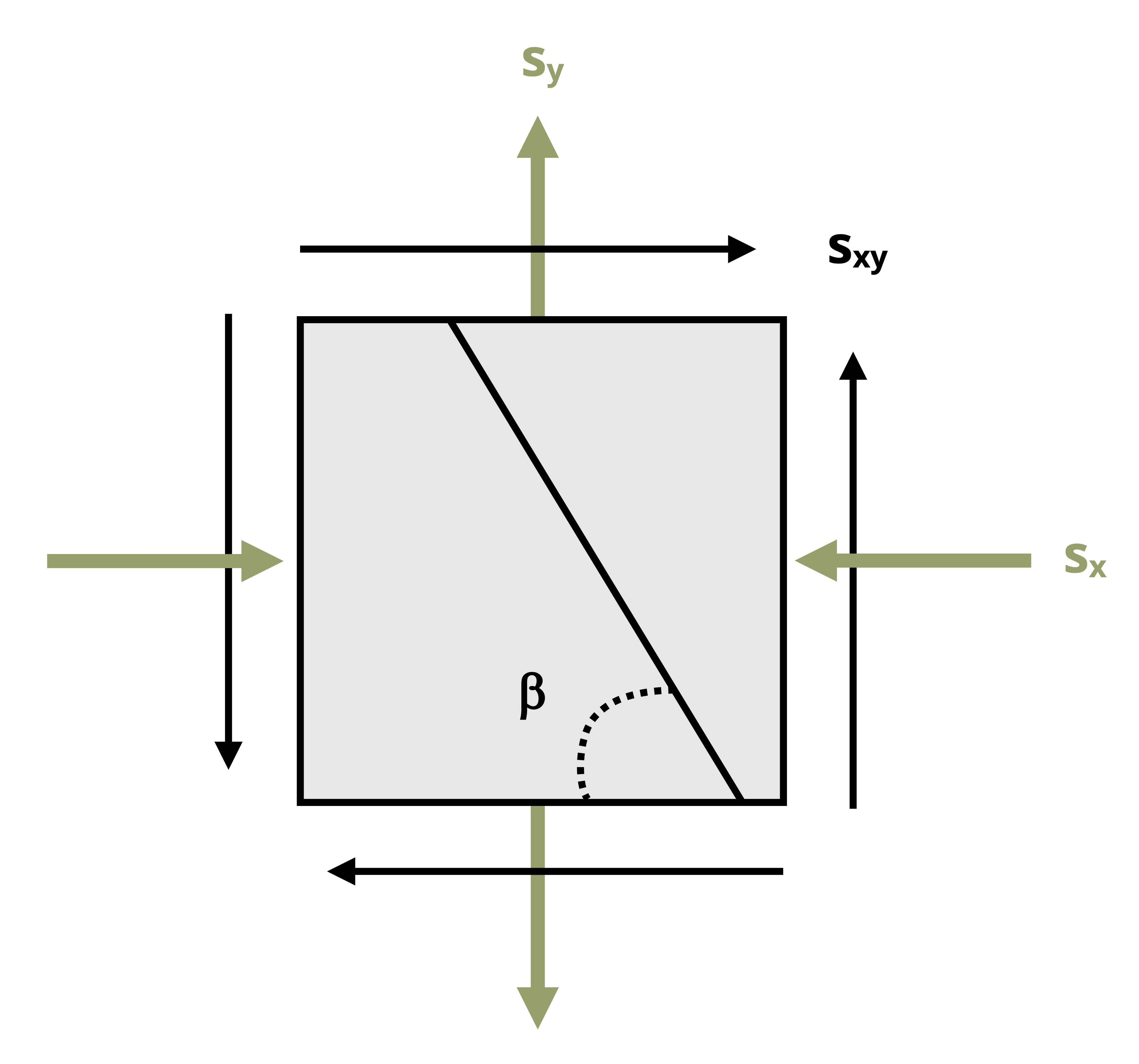
The general stress state at a point on a hollow pipe formed with spiral welds inclined to an angle β with respect to the horizontal is shown below. For stress magnitudes given as follows: Sx = 128 MPa, Sy = 80 MPa, Sxy = 75.45 MPa, and β = 42°. Determine the stress parallel and perpendicular to weld.
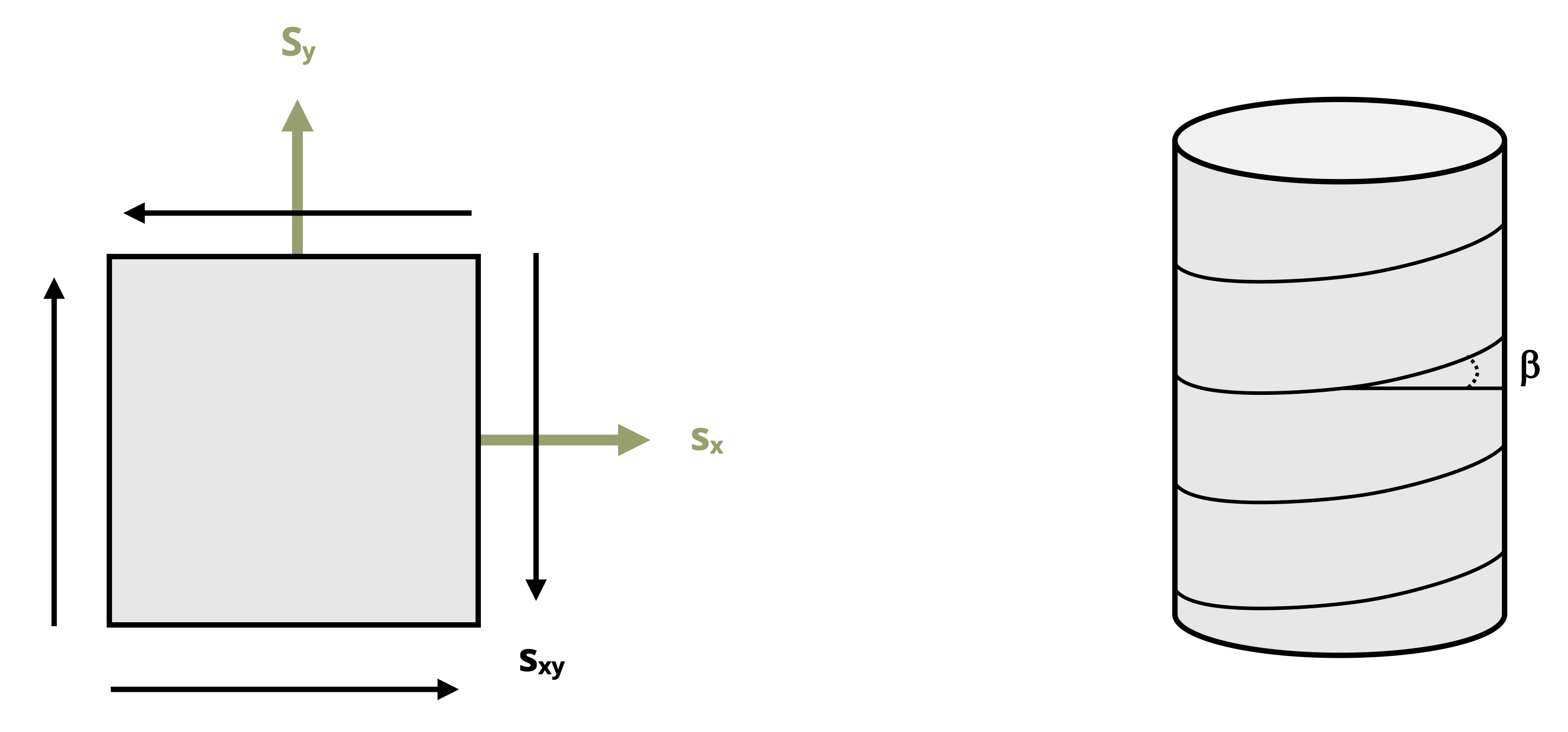
The stress parallel and perpendicular to the weld can be found by applying the stress transformation equations with σx = 128 MPa, σy = 80 MPa, and τxy = -75.45 MPa:
\[ \begin{aligned} & \sigma_n=\sigma_x \cos ^2(\theta)+\sigma_y \sin ^2(\theta)+2 \tau_{x y} \sin (\theta) \cos (\theta) \\ & \tau_{n t}=-\left(\sigma_x-\sigma_y\right) \cos (\theta) \sin (\theta)+\tau_{x y}\left(\cos ^2(\theta)-\sin ^2(\theta)\right) \end{aligned} \]
Notice that the normal stresses are positive since they are both shown to be tensile on the given stress element but the shear stress is negative based on the fact that the shear stress arrow goes in the negative y direction on the positive x-face (the same conclusion can be drawn by observing any of the other faces).
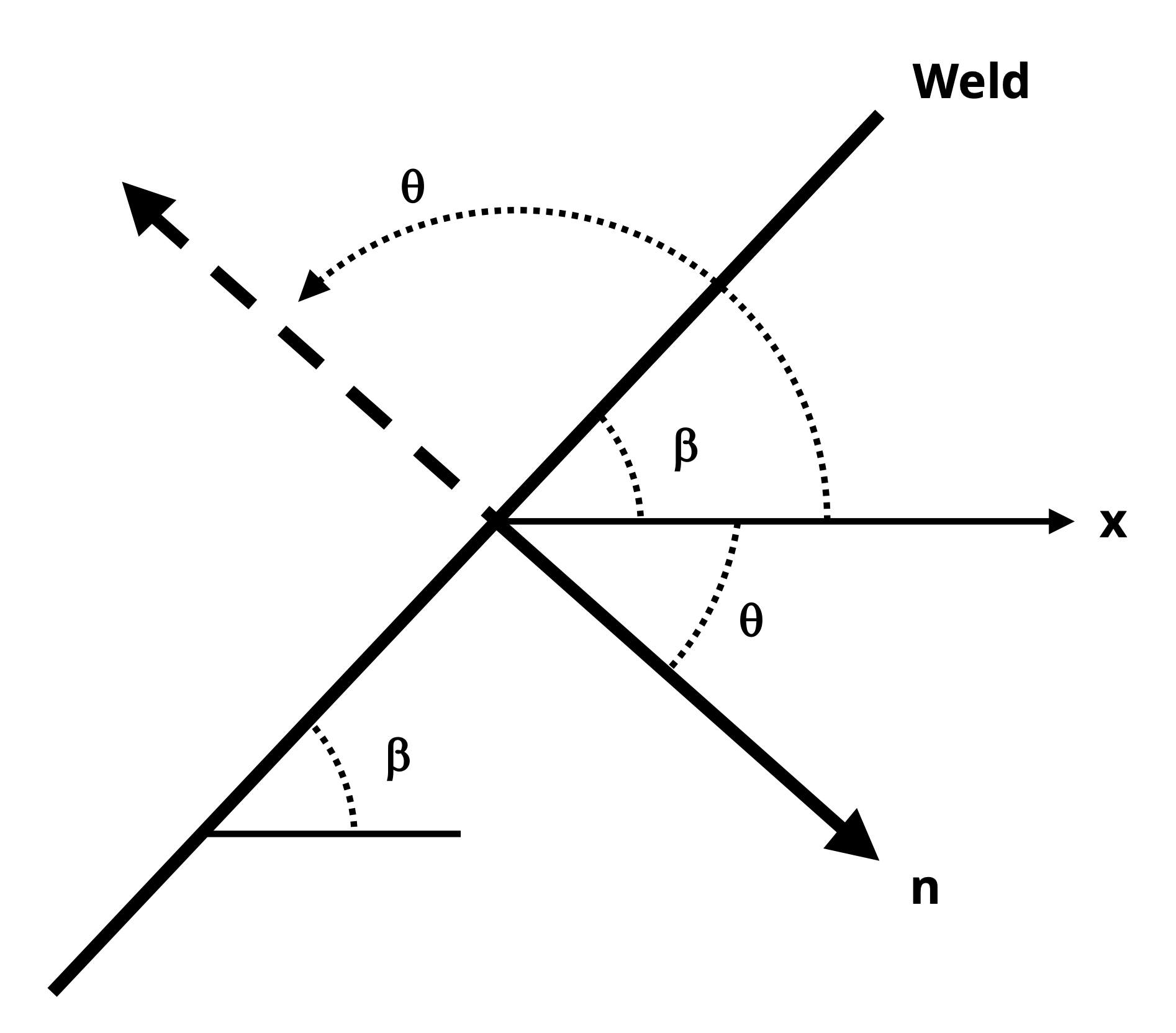
Before performing the calculation, the appropriate angle θ must also be found. The plane of interest in this as is the plane of the weld which is represented by the line representing the spiral. The angle θ needed to substitute into the equations is the angle between the x-axis and th normal axis to the weld. Based on the normal axis below the x-axis, we can see θ is θ = -(90 – β) = -48°. The angle is negative since it is a clockwise rotation to get from the x axis to the n-axis below.
We could also base θ on the dashed normal axis, in which case the magnitude of θ would be θ = 180° – 48° = 132°. This angle is positive since the rotation from the x-axis to the dashed normal axis is counterclockwise.
So with σx = 128 MPa, σy = 80 MPa, τxy = -75.45 MPa, and θ = -48° (or +132°), the stress normal to the weld is σn = 139.0 MPa. The stress parallel to the weld is τnt = 31.76 MPa.
Example 12.2
The stresses shown act at a point in a stressed body as shown. Normal and shear stress magnitudes acting on horizontal and vertical planes at the point are Sx = 1700 psi, Sy = 800 psi, and Sxy = 790 psi. Determine the normal (positive if tensile, negative if compressive) and shear stresses at this point on the inclined plane shown. Assume β = 36°.
We will first determine the angle θ that we need for the stress transformation equations. Recall the the process described in Section 12.1:
Draw a line that represents the plane of interest
Draw the x-axis positive going towards the right
Draw the axis normal to the plane of interest. It does not matter if you draw the normal axis as oriented counterclockwise or clockwise from the x-axis as long as you use the correct sign for the angle (see step 4).
Determine the angle that goes from the x-axis to the normal axis. This angle is θ. If the direction from the x-axis to the normal axis is counterclockwise, then θ should be taken to be positive. If the direction from the x-axis to the normal axis is clockwise, then θ should be taken to be negative.
Either angle labeled θ in the illustration will work and produce the same results. In this example, we will use the smaller of the two:
θ = 90 – β = 54°.
The angle is positive since the n-axis is rotated counterclockwise from the positive x-axis.
With θ determined, the only thing left to do is make the subsitutions into the stress transformation equations and calculate. Note that the σn equation will give us the normal stress on the rotated x-face (x’), so will need to also calculate σn with the angle (θ + 90°) to get σy’ or use the stress invariance concept: (σx + σy = σx’ + σy’)
Substituting σx = -1700 psi (negative since it is shown to be compressive), σy = 800 psi, τxy = 790 psi, and θ = 54° into:
\[ \begin{aligned} & \sigma_n=\frac{\sigma_x+\sigma_y}{2}+\frac{\sigma_x-\sigma_y}{2} \cos (2 \theta)+\tau_{x y} \sin (2 \theta) \\ & \tau_{n t}=-\frac{\sigma_x-\sigma_y}{2} \sin (2 \theta)+\tau_{x y} \cos (2 \theta) \end{aligned} \]
Gives σx’ = 687.6 psi and τx’y’ = 945 psi.
Furthermore, applying stress invariance: -1700 psi + 800 psi = 687.6 psi + σy’ gives σy’ = -1588 psi
σx’ = 687.6 psi
τx’y’ = 945 psi
σy’ = -1588 psi
12.2 Principal Stresses and Max/Min Shear Stress
Click to expand
Often, the plane we would be the most concerned with is the one on which the normal stress or the shear stress is at a maximum or minimum. The maximum and minimum normal stresses are referred to as the principal stresses (σ1 and σ2) and the planes on which they act (described by angle of rotation of the stress element, θp1 and θp2) are the principal planes. The maximum and minimum shear stresses are simply referred to as the maximum and minimum shear stress, respectively, and the planes on which they occur are referred to simply as the planes of maximum and minimum shear stress (denoted as θs1 and θs2).
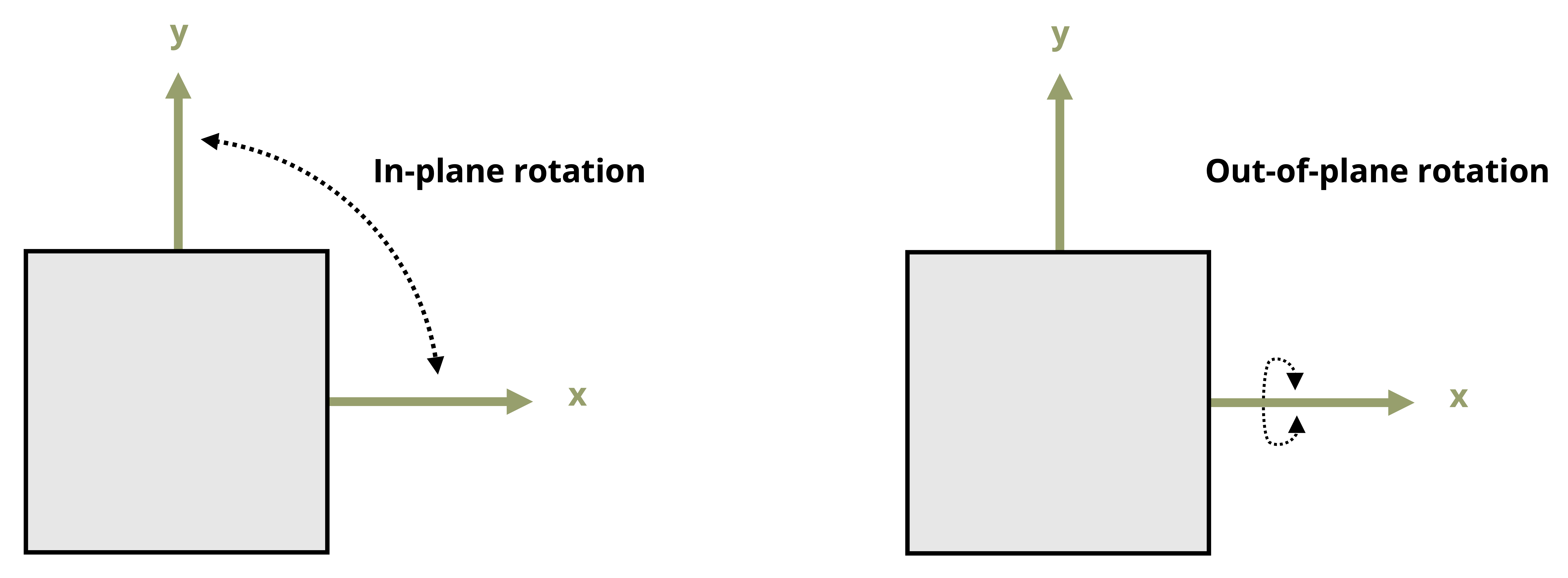
It is important to note that in this section, only rotations within a two dimensional plane are being considered. As will be seen in Section 12.4, the principal planes and principal stresses are the same even when considering out of plane rotation of the stress element (see Figure 12.7), but the max shear stress could be different. Therefore, the max and min sheer stress as determined by the below derived equations will be referred to as the max/min in-plane shear stress.
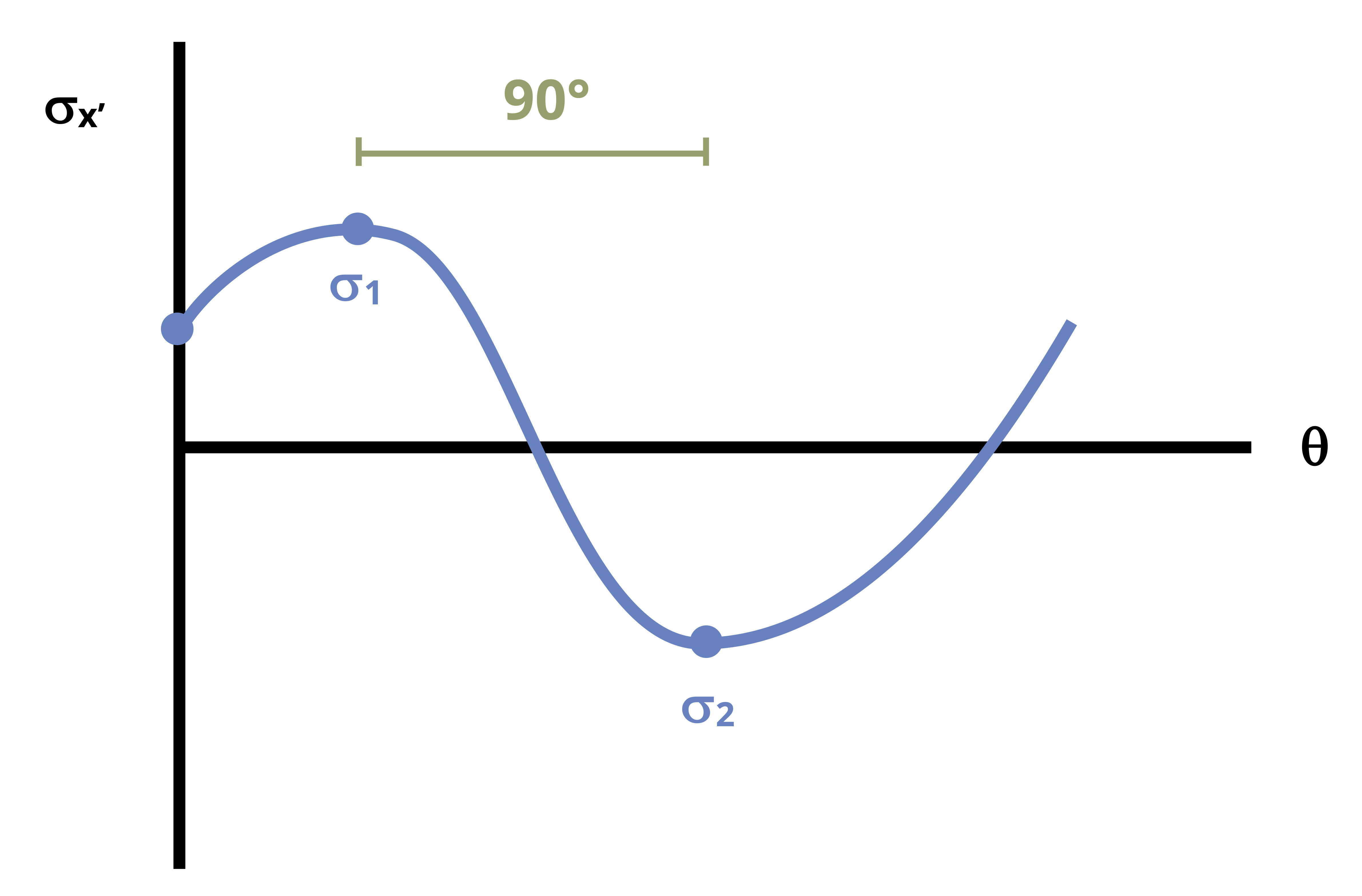
As we rotate the stress element and the angle θ changes, the stress changes in a predictable way. Figure 12.8 shows the variation of normal stress σx’ with angle θ. The principal stresses can be seen to occur at specific values of θ. These angles will be 90° apart from one another. A similar graph could be drawn for τx’y’.
Since these stresses are maximums and minimums (i.e., the slope of the curve is zero at these points) and since the transformation equations derived in Section 12.1 are functions in terms of the plane rotation angle θ, we can simply take the derivates of the two equations and set them equal to zero to find the angles at which we would get the maximum and minimum of each type of stress. Using the second set of transformation equations derived in Section 12.1 (though the first set would yield the same results):
\[ \begin{aligned} & \frac{d \sigma_n}{d \theta}=-\left(\sigma_x-\sigma_y\right) \sin \left(2 \theta_p\right)+2 \tau_{x y} \cos \left(2 \theta_p\right)=0 \\ & \frac{d \tau_{n t}}{d \theta}=-\left(\sigma_x-\sigma_y\right) \cos \left(2 \theta_s\right)-2 \tau_{x y} \sin \left(2 \theta_s\right)=0 \end{aligned} \]
Notice that θ is subscripted with a p in the first equation since this theta represents a principal plane as defined above. Similarly, θ is subscripted with and S in the second equation since this theta represents a plane of max or min in-plane shear stress.
These equations can be rearranged to isolate Tan (2θ) on one side and subsequently used to find θp and θs values:
\[ \boxed{\begin{aligned} \tan \left(2 \theta_p\right) & =\frac{2 \tau_{x y}}{\left(\sigma_x-\sigma_y\right)} \\ \tan \left(2 \theta_s\right) & =-\frac{\left(\sigma_x-\sigma_y\right)}{2 \tau_{x y}} \end{aligned}} \tag{12.2}\]
𝜃p = Orientation of one of the principal planes, with respect to the x-axis [\(^\circ\), rad]
𝜃s = Orientation of one of the maximum shear planes, with respect to the x-axis [\(^\circ\), rad]
𝜏xy = Average shear stress in the xy plane, prior to any transformation [Pa, psi]
𝜎x = Average normal stress in the x-direction, prior to any transformation [Pa, psi]
𝜎y = Average normal stress in the y-direction, prior to any transformation [Pa, psi]
Once the angles associated with the planes of extreme stresses are determined, they can be substituted into the stress transformation equation of Section 12.1 along with the stresses in the given plane to find the principal stresses and max/min shear stress.
A few calculation details that it will be helpful to remember are:
The inverse tangent function has two possible solutions. One solution would be the angle that will be reported by a calculator, and the other possible answer is the angle that is that angle plus or minus 180°. So if you use your calculator to solve the Tan (2θp) equation, you would take half that to get the first principle angle and then add or subtract 90 degrees to that principal angle to get the second. The same idea applies to finding the two θs angles.
By convention, the most positive of the two principal stresses is denoted as σ1. The other principal stress is then σ2. The angle that produces that σ1 stress is θp1 and the angle that produces σ2 is θp2.
The max and min in-plane shear stresses will always turn out to be equal in magnitude by opposite in sign, or in other words, the minimum shear stress is always the negative of the maximum shear stress. As with the principal planes and stresses, one would need to substitute one of the θs angles into the shear stress transformation equation to determine which angle corresponds to the maximum in-plane shear stress and which corresponds to the minimum.
The angles of maximum and minimum shear stresses are 90° apart from each other, and 45° apart from the principal directions. If one principal direction is found to be, for example, 40° then the other principal direction can be determined as either (40° + 90° =) 130° or (40° - 90° =) -50°. The angles of maximum and minimum in-plane shear stress can then be determined as either (40° + 45° =) 95° or (40° - 45° =) - 5°. It is also acceptable to add or subtract 45° from 130° or from – 50°.
Given the variety of different of possible correct angles, we will use a convention that principal directions and angles of maximum and minimum shear stress will be calculated in the range – 90° ≤ θ ≤ + 90°.
If desired, the principal stresses and max./min. shear stresses can be calculated directly without first finding the principal directions:
\[ \boxed{\begin{gathered} \sigma_{1,2}=\frac{\sigma_x+\sigma_y}{2} \pm \sqrt{\left(\frac{\sigma_x-\sigma_y}{2}\right)^2+\tau_{x y}{ }^2} \\ \tau_{x \prime y^{\prime}}= \pm \sqrt{\left(\frac{\sigma_x-\sigma_y}{2}\right)^2+\tau_{x y}{ }^2} \end{gathered}} \tag{12.3}\]
𝜎1,2 = Principal stresses [Pa, psi]
𝜎x = Average normal stress in the x-direction, prior to any transformation [Pa, psi]
𝜎y = Average normal stress in the y-direction, prior to any transformation [Pa, psi]
𝜏xy = Average shear stress in the xy plane, prior to any transformation [Pa, psi]
Some useful conclusions that can be drawn simply by studying the principal plane and plane of max/min shear stress equations are as follows:
If the shear stress transformation equation given in Section 12.1 is set equal to 0 in order to find the plane at which shear stress is equal to 0, we would arrive at the same equation as the Tan(2θp) found above. We can then conclude that shear stress is 0 on the principal planes. It can also be said that if the shear stress is found to be 0 on any given plane, then that plane must be a principal plane.
The equation for Tan(2θs) is the negative inverse of the equation for Tan (2θp). This means that 2θs = 2θp ± 90° or θs = θp ± 45°. Recognizing this can allow one to calculate one set of angles more efficiently once the other is found.
If either of the θs angles are substituted into the normal stress transformation equation, the normal stress would work out to be the average stress \(\left(\frac{\sigma_x+\sigma_y}{2}\right)\). Once again, this recognition can help make determining the total stress state on the plane of max/min shear stress more efficient.
Example 12.3 demonstrates the calculation of the principal stresses, the maximum in-plane shear stress, and the orientations that these stresses occur at.
Example 12.3
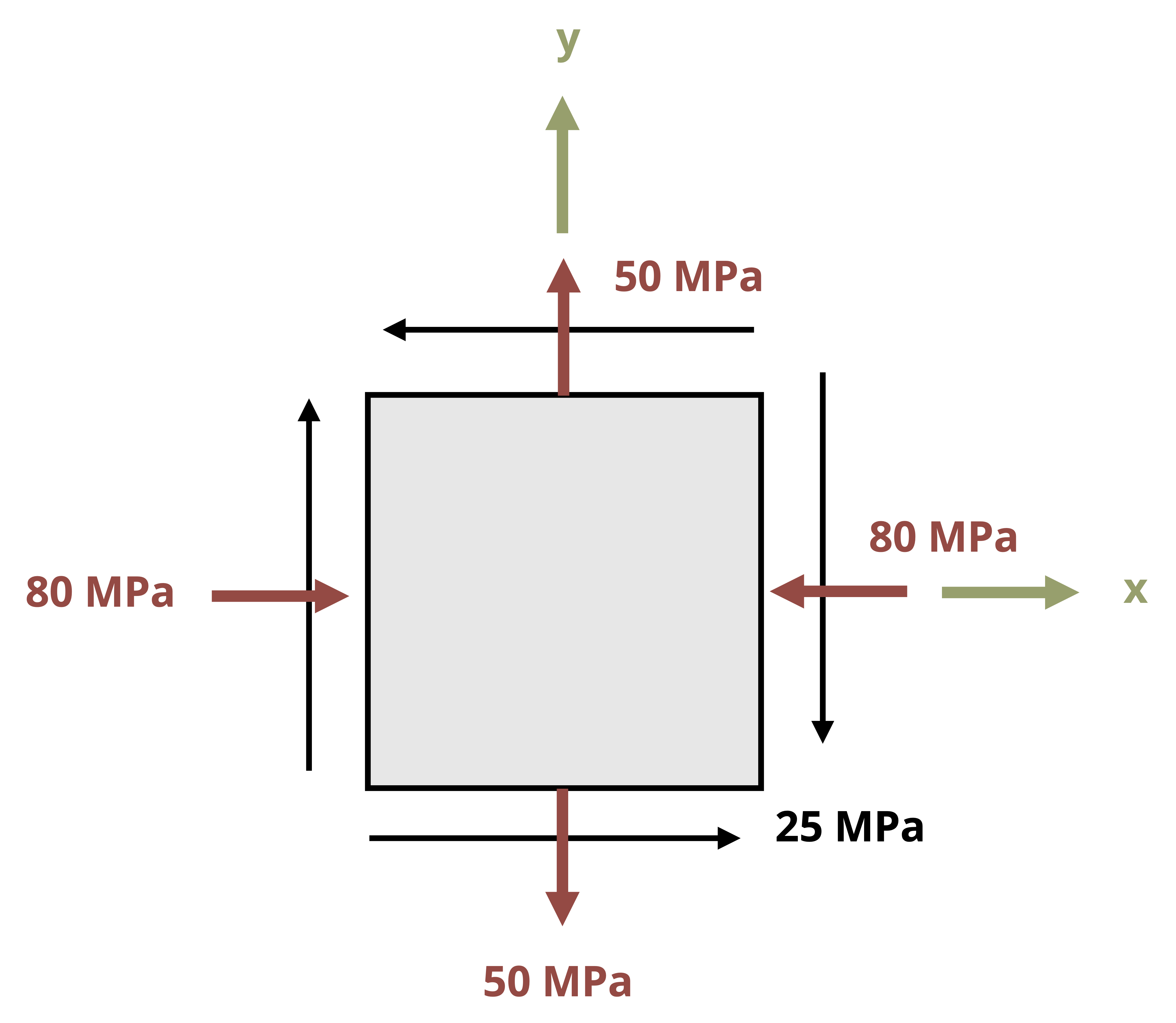
The state of plane stress at a point is represented by the stress element below. Determine the principal stresses and the maximum in-plane shear stress and draw the corresponding stress elements.
Following the steps given at the end of Section 12.2:
Find the principal planes using
\[ \operatorname{Tan}\left(2 \theta_p\right)=\frac{2 \tau_{x y}}{\left(\sigma_x-\sigma_y\right)} \]
With σx = -80 MPa, σy = 50 MPa, and τxy = -25 MPa, we get:θp = 10.52° based on the answer from the calculator.
The other angle is then θp = 10.52° + 90° = 100.52°
So the principal plane angles are 10.52° and 100.52°.
Subbing θp = 10.52° into:
\[ \sigma_n=\frac{\sigma_x+\sigma_y}{2}+\frac{\sigma_x-\sigma_y}{2} \cos (2 \theta)+\tau_{x y} \sin (2 \theta) \]gives σn = -84.6 MPa and subbing θp = 100.52° in gives σn = 54.6 MPa.
Since 54.6 MPa is the most positive of the two principal stresses, σ1 = 54.6 MPa and σ2 = -84.6 MPa.
The 54.6 MPa would go on the rotated x-face and the -85.6 MPa would go on the rotated y-face of the stress element rotated counterclockwise 100.52°.
Conversely, if the stress element is rotated counterclockwise by 10.52°, the stress on the rotated x-face would be -84.6 MPa and the stress on the rotated y-face would be 54.6 MPa.Drawing the stress element rotated to the principal planes:
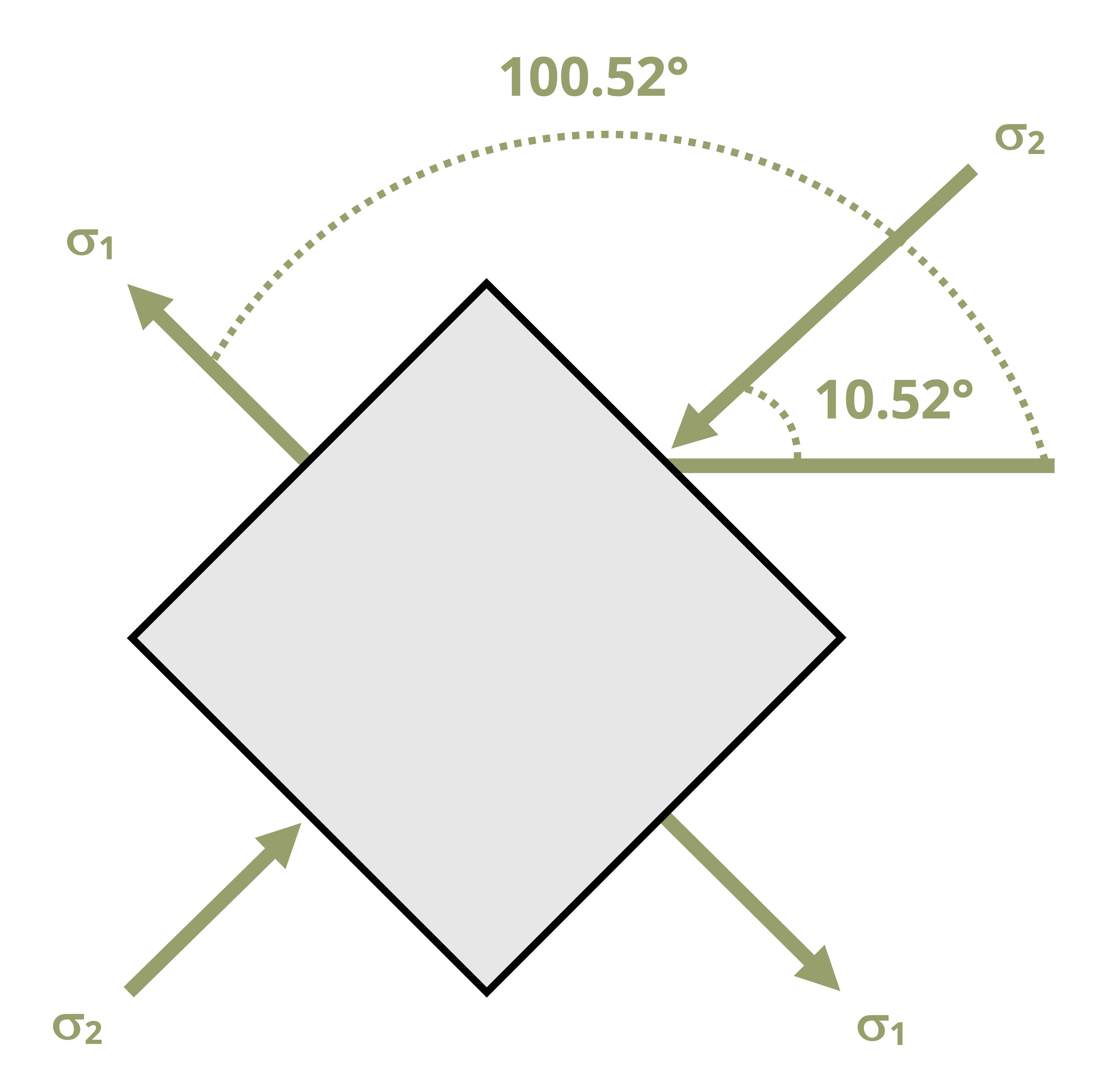
Notice that the stress element looks the same no matter which angle is used for the rotation. Also note that the shear stress on the principal plane is 0.Next we will find the planes of max/min in-plane shear planes as well as the corresponding shear stresses. We could use:
\[ \operatorname{Tan}\left(2 \theta_s\right)=-\frac{\left(\sigma_x-\sigma_y\right)}{2 \tau_{x y}} \]But since we already have the θp angles, we will use the fact that the max/min in-plane shear stress planes are +/- 45° from those. We can choose either θp angle to add and subtract the 45° to and from. The final orientation of the element would be the same. Since it is generally easier to visualize angle rotations smaller in magnitude than 90, so we will use the smaller θp value.
So θs = 10.52° +/- 45° = 55.5° and -34.5°.Subbing θs = 55.5° into:
\[ \tau_{n t}=-\frac{\sigma_x-\sigma_y}{2} \sin (2 \theta)+\tau_{x y} \cos (2 \theta) \]gives τnt = 69.6 MPa. Since this is a positive value, we know that this is the max in-plane shear stress and that θs = -34.5 ° should give τnt = -69.6 MPa = τmin (in-plane).
So if we rotate the stress element counterclockwise by 55.5°, we would draw a positive shear stress and if we rotate it clockwise 34.5 degrees, we would draw a negative shear stress.
The normal stress on the plane of max/min in-plane shear stress is
\[ \sigma=\sigma_{avg}=\frac{\left(\sigma_x+\sigma_y\right)}{2}=-15 \mathrm{MPa} \]
Drawing the stress rotated to the planes of max/min shear stress:
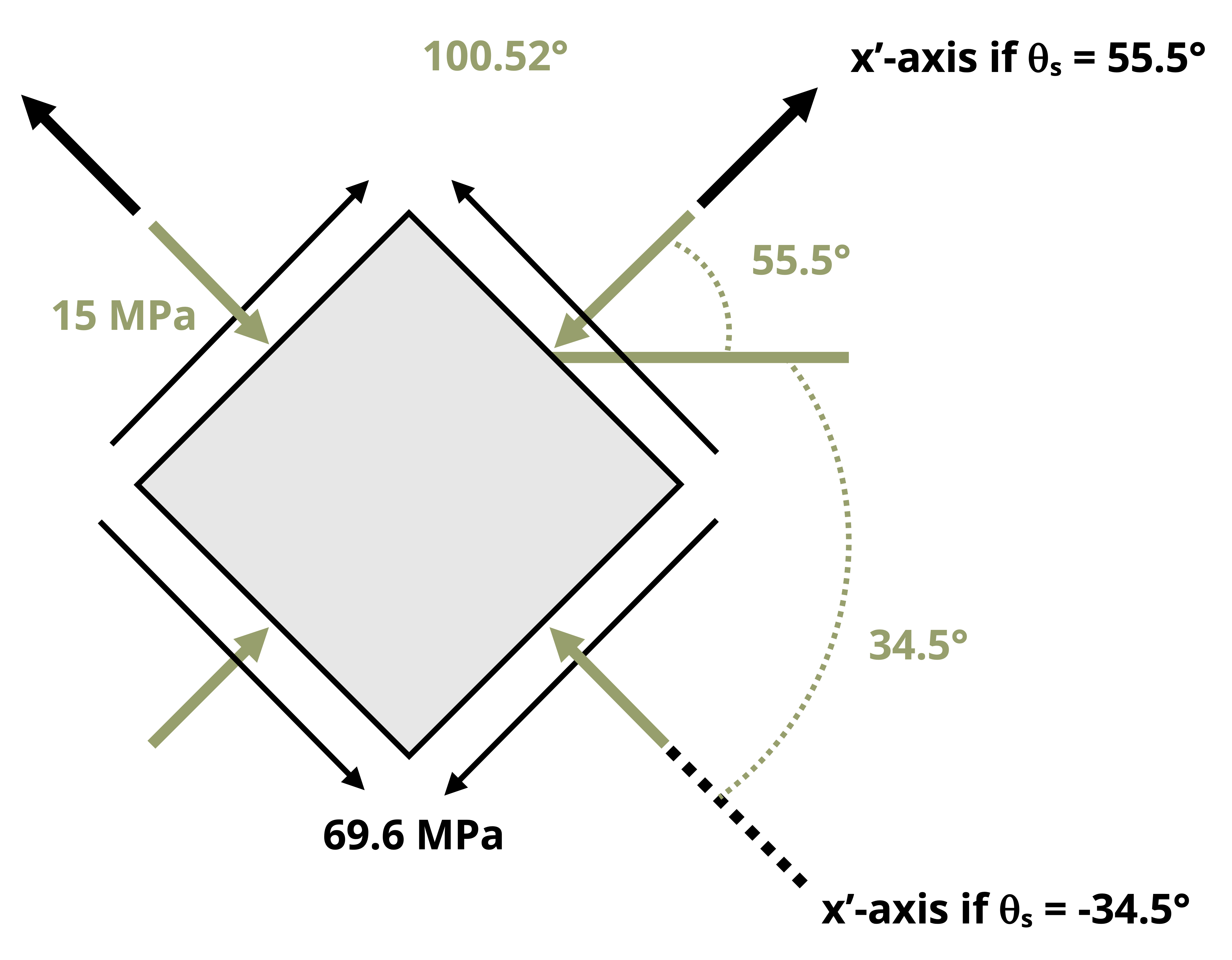
Once again, notice that the stress element looks fundamentally the same regardless of which θs angle is used.
θp1 = 100.52° and θp2 = 10.52°
σ1 = 54.6 MPa and σ2 = - 84.6 MPa
θs = 55.5° and -34.5°
τmax (in-plane) = 69.6 MPa
τmin (in-plane) = - 69.6 MPa
Elements are drawn above.
12.3 Mohr’s Circle
Click to expand
As an alternative to using equations to determine principal planes and stresses as well as max/min shear planes and stresses, one can use a graphical method known as Mohr’s Circle. The stress transformation equations can be seen to actually be equations of a circle where the perimeter of the circle consists of coordinates points that correspond to normal stress on the horizontal axis and shear stress on the vertical axis. The advantage of using Mohr’s Circle is that it does not involve needing to recall equations and can be quick and efficient to use with some practice.
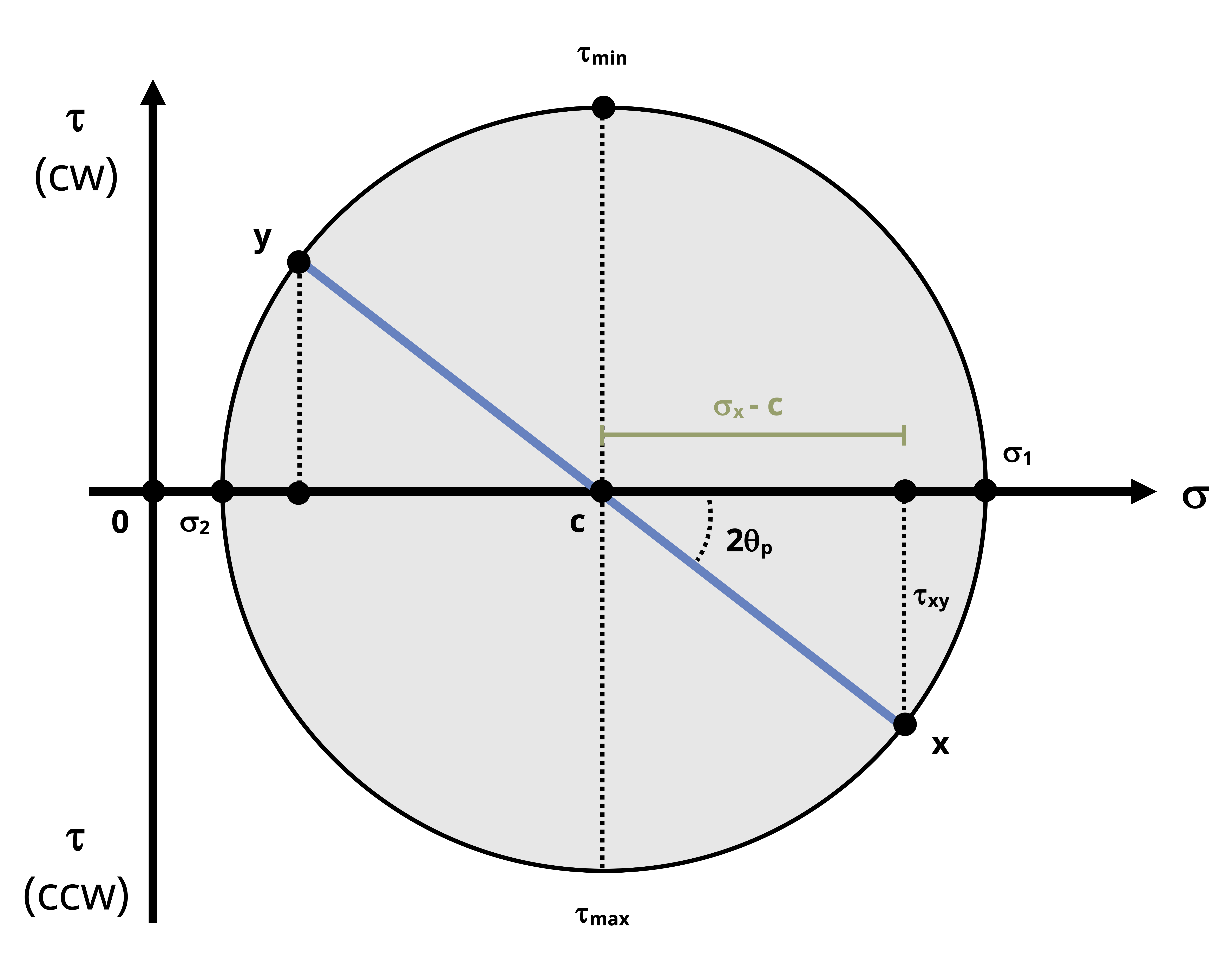
To construct the circle (refer to the fully constructed Mohr’s circle in Figure 12.11):
To start, draw a set of coordinate axes where normal stress will be on the horizontal axis and shear stress will be on horizontal axis. Note in 12.9 that the shear stress is labeled with a (CW) for clockwise on the positive side and a (CCW) for counterclockwise on the negative side as a reminder of how the signs on the vertical coordinates are determined.
Plot the center of the circle, C, which will lie on the normal stress axis at a point equal to the average normal stress.
\[ C=\left(\frac{\sigma_x+\sigma_y}{2}, 0\right) \]Next, one coordinate point on the circle needs to be established based on the given stress state and plotted on the axes. This point, which we will call the x-point, will come from the stresses drawn on the positive x-face of the stress element. The normal stress is positive if tensile and negative if compressive. The sign on the vertical coordinate, the shear stress, will depend on the direction of rotation that the shear stress on the x-face will cause. If it would tend to rotate the element clockwise, it will be plotted on the positive side of the vertical axis and vice versa.
On the representative stress element in Figure 12.9 below, the normal stress on the x face is tensile and the upwards shear stress would tend to cause the element rotate counterclockwise, so the x-point is (+σx, -τxy).
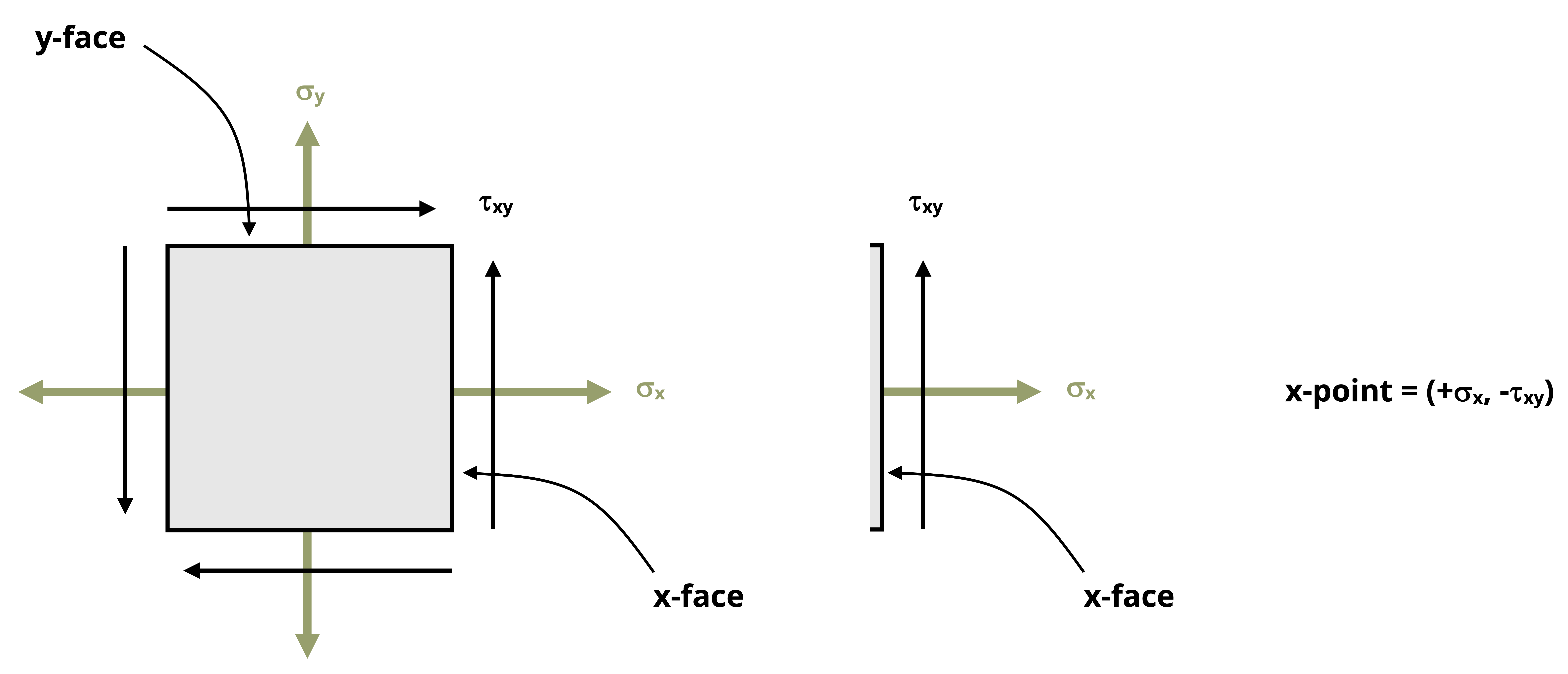
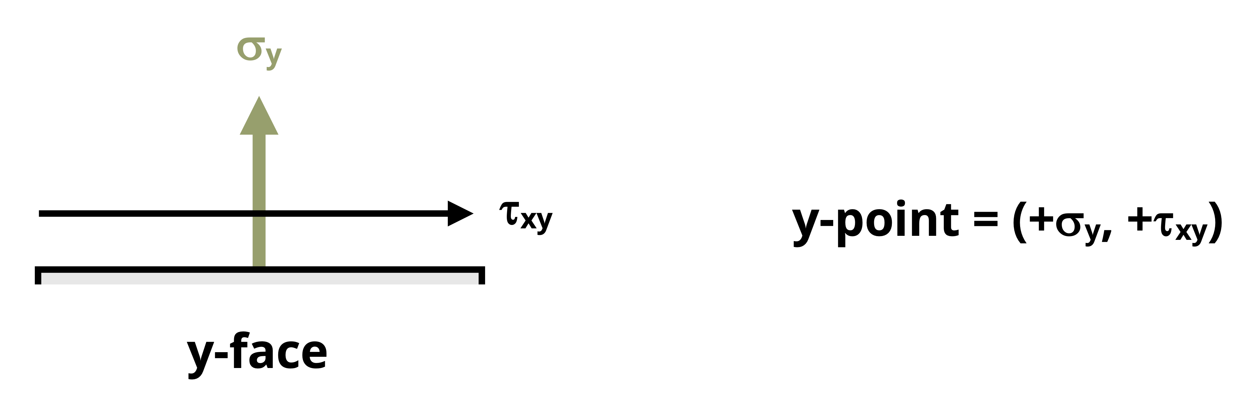
We could alternatively use what we will call the y-point, which comes from the stresses acting on the positive y-face of the stress element with the same sign conventions above. For the representative stress element of Figure 12.9, the normal stress on the y face (Figure 12.10) is drawn in the tensile direction and the rightwards shear stress would tend to cause the element to rotate clockwise, so the y-point is (+σy, +τxy).
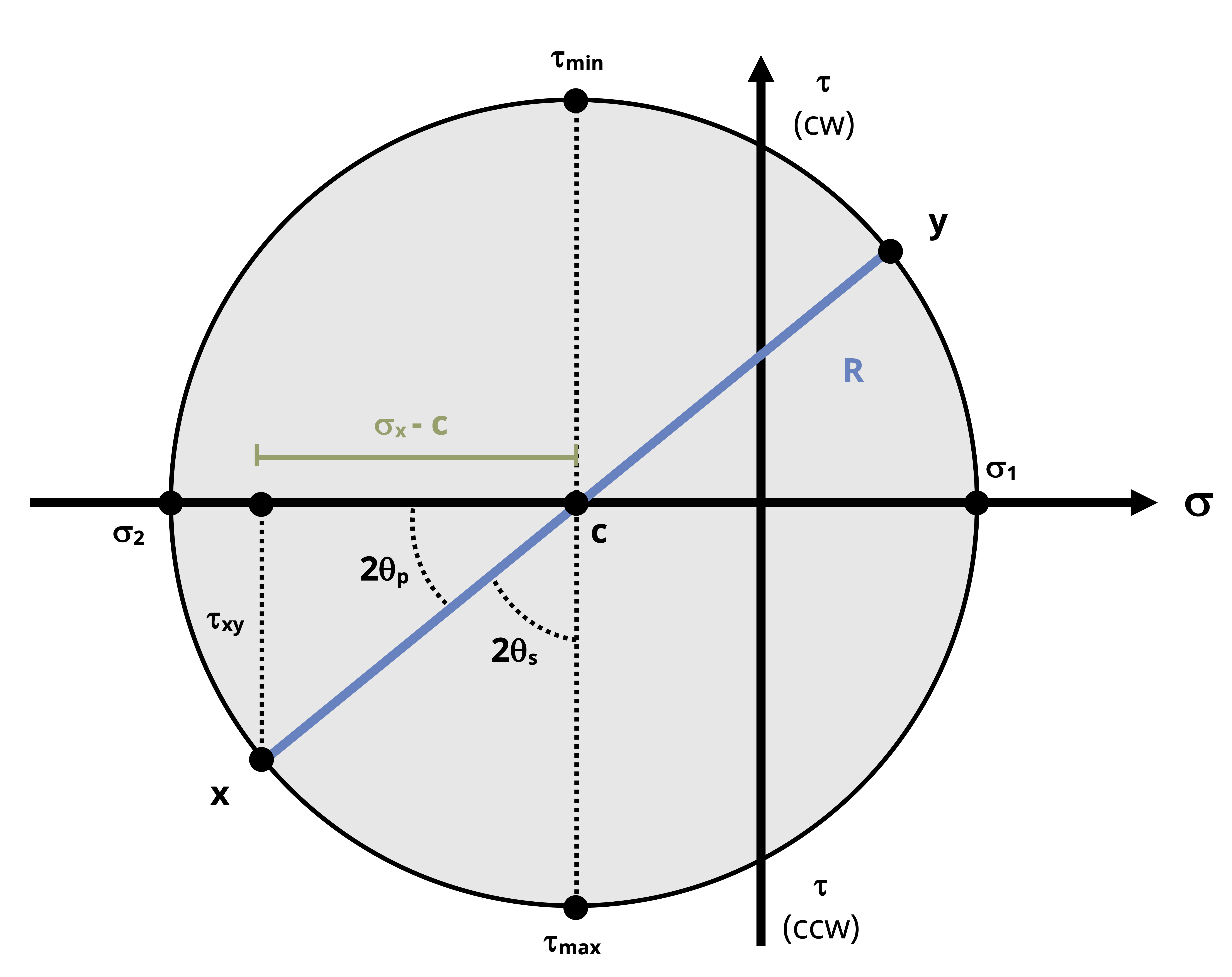
Once the center and either the x-point or y-point are plotted, draw a line that connects them. This line is the radius of the circle. This radius, R, can be determined using of the Pythagorean Theorem on the triangle formed between C, σx, and the x-point. Since the radius of the circle will be constant, we can now draw the rest of the circle.
\[ R=\sqrt{\left(\sigma_x-C\right)^2+\tau_{x y}^2} \]Recalling that the shear stress is zero on the principal plane, we can observe that that corresponds exactly to the normal stress axis so we can identify σ1 to be the normal stress on the right extreme of the circle and σ2 to be the normal stress on the left extreme of the circle. Furthermore, based on inspection of the circle and the known points, we can see that σ1 = C + R and σ2 = C - R.
It can also be seen that the max and min in-plane shear stress would be at the bottom and top of the circle, respectively, so we can say that τmax = +R and τmin = -R.
The max shear stress is at the bottom since a positive shear stress on the positive x-face would cause the stress element to rotate counterclockwise.
The circle also confirms that the normal stress on the plane of max/min in-plane shear stress is \(\mathrm{C}=\sigma_{avg}=\frac{\sigma_x+\sigma_y}{2}\)
To find the angles of the principal planes and max/min shear stress, or to use the circle to perform stress transformations to arbitrary planes, one must note that rotations around the circle represent twice the actual amount of rotation required to get from the stress state in one plane to the stress state in the rotated plane. Furthermore, rotations counterclockwise from the x-point are considered to be positive angles and the rotations clockwise from the x-point are considered to be negative angles.
Thus, the angle between the radial line that connects C and the x-point to the principal plane (normal stress axis) is 2θp. This angle can be determined by applying right triangle trigonometry principles to the right triangle used to find the radius:
\[ \tan (2 \theta p)=\frac{C+\sigma_x}{\tau_{x y}} \]
As discussed in Section 12.2, the inverse tangent function will have two solutions. One of those solutions (divided by 2) will be the angle that corresponds to rotating from the x point to the σ1 side of the circle from which means that this principal angle leads to σ1 acting on the rotated x face (x’ face) of the stress element and therefore σ2 acts on the rotated y face (y’ face). The other solution to θp will correspond to the angle necessary to rotate from the x point to the σ2 side of the circle which will lead to σ2 acting on the x’ face and σ1 acting on the y’ face.The angle to the plane of max/min in-plane shear stress can be found in a similar manner. By visual inspection one can see that the tan(2θs) will be the inverse of tan(2θp). Alternatively, it can be calculated as 2θs = 90° - 2θp. One should note, however, the directions of the angles for rotation. Recalling the convention used to apply sign to the shear stress coordinate, the angle that goes from the x-point to the negative side of the shear stress axis will correspond to the rotation that results in the maximum in-plane shear stress and vice versa.
Once these quantities are known, the use of the circle to perform stress transformations at arbitrary planes requires making similar trigonometric calculations. This process is better illustrated in Example 12.4.
12.4 Mohr’s Circle in 3-Dimensions and Absolute Max Shear Stress
Click to expand
The methods discussed so far in Sections 12.2 and 12.3 provide the maximum in-plane shear stress that arises from planar rotations in the 2D plane, but as discussed in Section 12.2, the actual maximum shear stress may result from an out of plane rotation. Thus, while this text is generally restricted to planar (2D) stress states, we need to consider a 3D stress element in order to determine the absolute maximum shear stress.
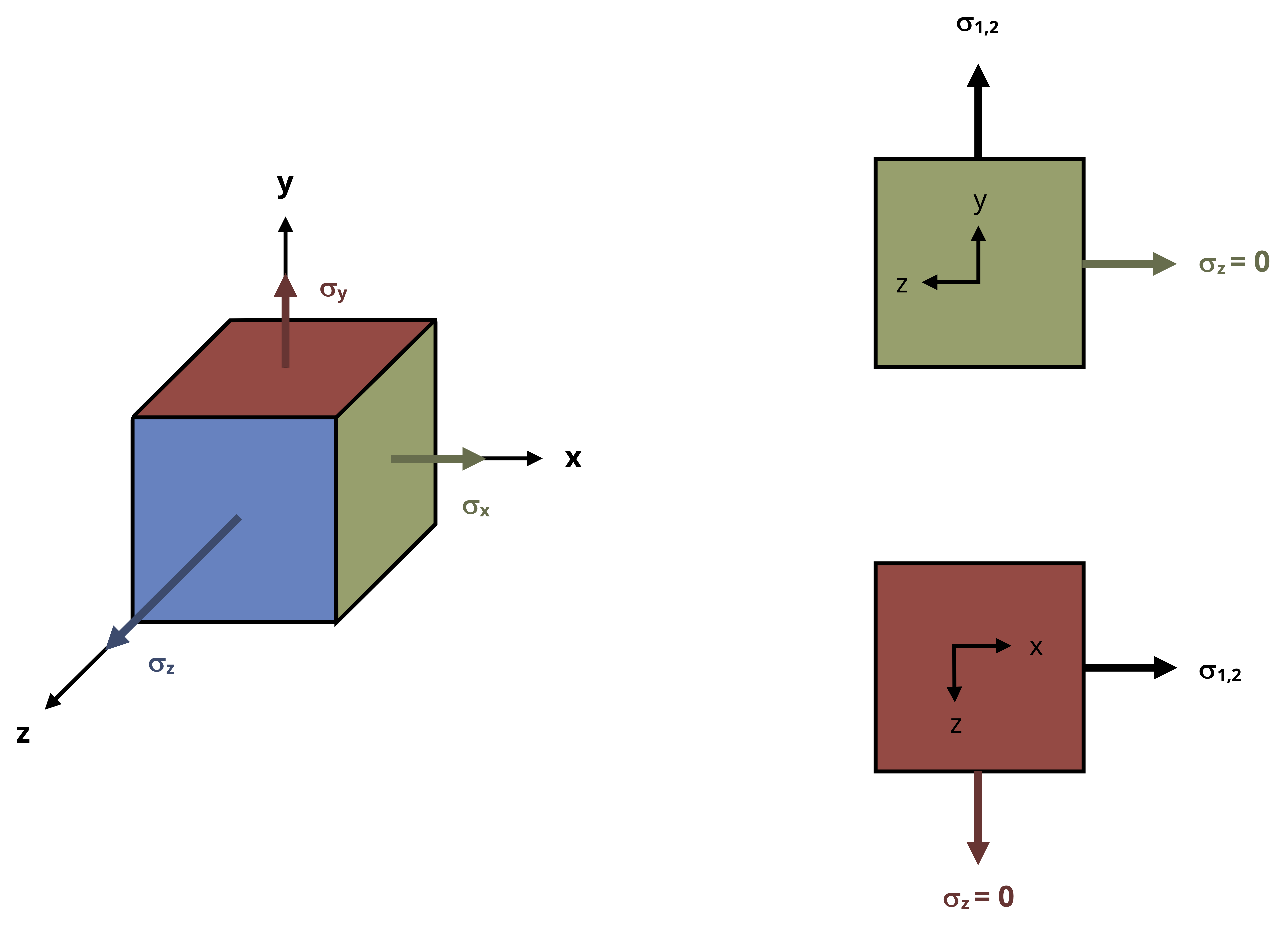
However, we are still considering only cases in which the stresses act in just two of the three principal directions. For the sake of this discussion, we will say that the stresses act in only the x and y directions, though it could generally be any combination of two axes. If stresses act only in the x and y directions, then a 3D stress element would include these stresses on the x and y faces, but the normal stress on the z face would be zero and the shear stress in the xz and yz planes would also be zero (see Figure 12.12). Recalling the earlier finding that if the shear stress is 0 on a given plane, the plane is a principal plane, we can say that the xz plane and the yz planes are principal planes with respect to rotation of the element around the y and x axes respectively.
It we start with the stress element already rotated in the xy plane to one of its principal planes, we know that the stresses on the x and y faces in this plane (x’ and y’ faces) will be σ1 and σ2 or vice versa. This means that σ1 (or σ2) and σz are the principal stresses on the yz plane and the σ1 (or σ2) and σz are the principal stresses on the xz plane. Since we are still dealing with plane stress, we know that σz = 0. In the case of plane stress then, there are principal stresses σ1 and σ2 as above, as well as σ3 = 0.
We can draw Mohr’s circle for each of these three planes on one plot. We will consider three cases:
σ1 and σ2 on based on the xy plane are both positive
σ1 and σ2 on based on the xy plane are both negative
σ1 and σ2 on based on the xy plane are opposite signs
Case 1:
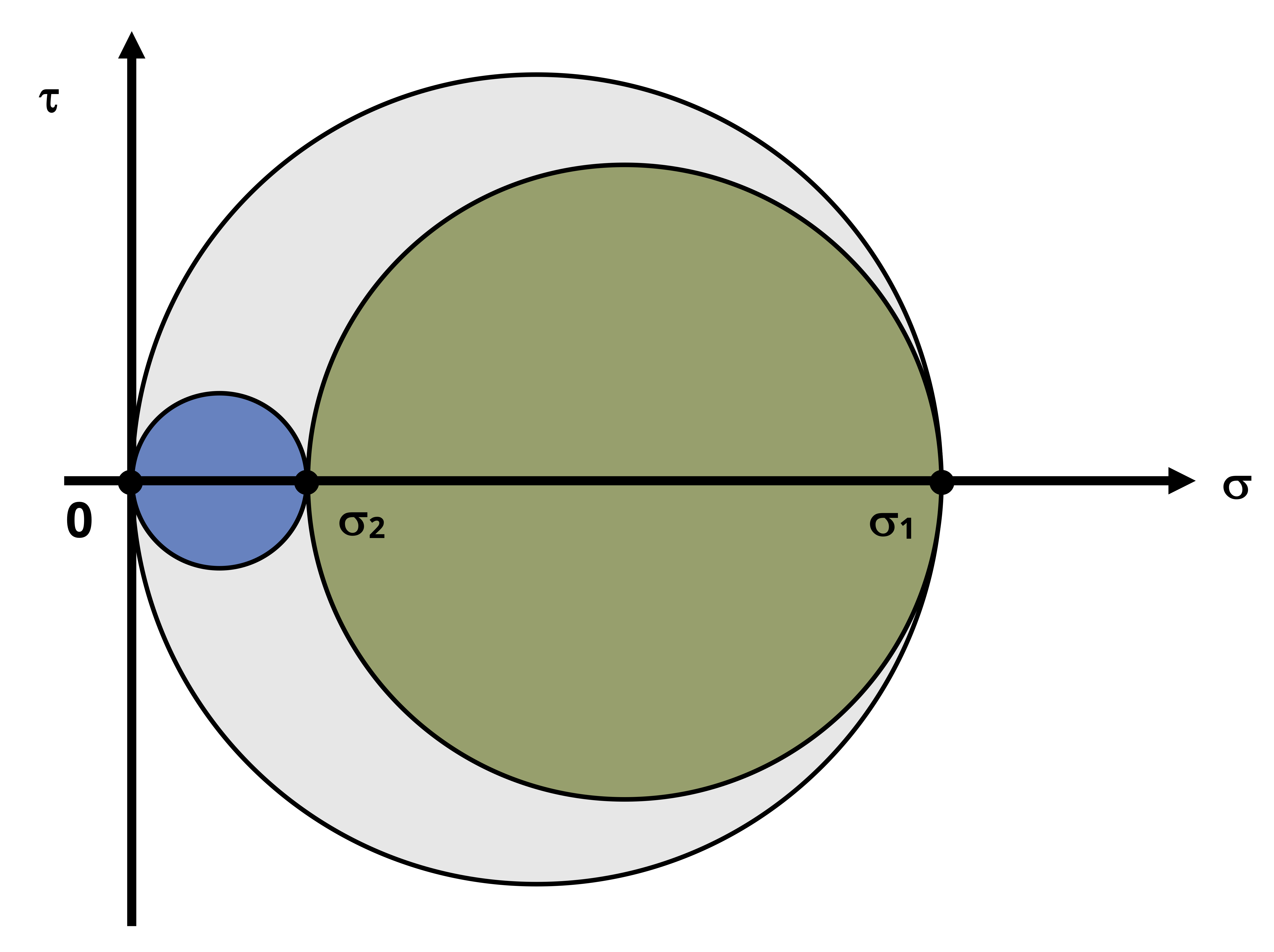
Referring to Figure 12.13, the larger inner circle is Mohr’s circle for the x-y plane as can be noted by the fact that the max and min normal stresses on that circle are σ1 and σ2, respectively. The smaller inner circle is Mohr’s circle for either the x-z or the y-z plane (whichever one has σ2 as the principal stress on the non-z face). The largest circle is Mohr’s circle for the other of the two non xy planes. We can see in this case that the largest shear stress is given by the radius of the largest circle which is σ1/2.
So in the case that σ1 and σ2 are both positive, the absolute max shear stress is:
\[ \tau_{(\max )absolute}=\left|\frac{\sigma_1}{2}\right| \]
The absolute value is there since we now the max shear stress must be a positive shear stress given that the max and min shear stresses are negatives of each other.
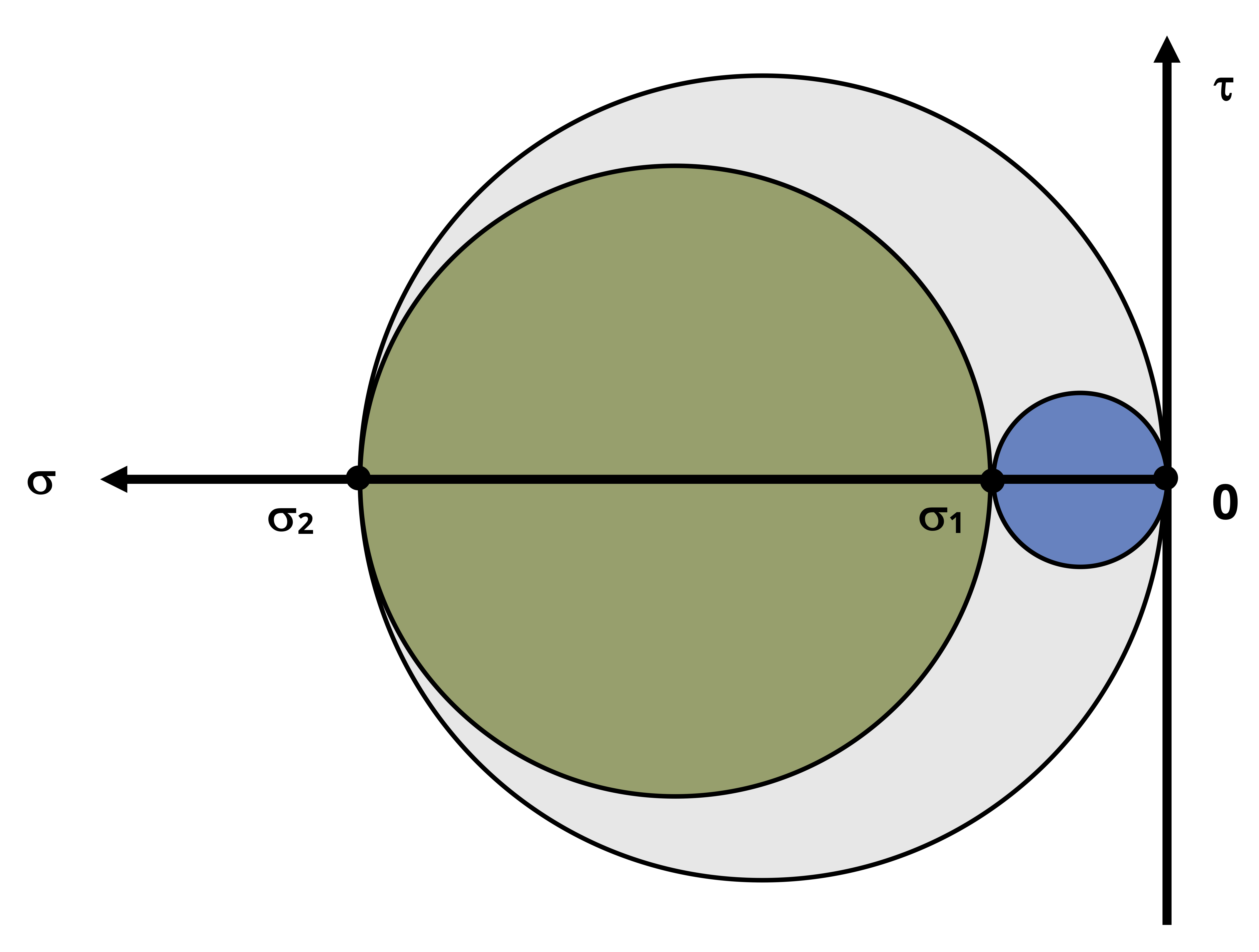
Case 2:
Referring to Figure 12.14, all the statements made in Case 1 still hold true except that the radius of the largest circle is now σ2/2.
So in the case that σ1 and σ2 are both positive, the absolute max shear stress is:
\[ \tau_{(\max )absolute}=\left|\frac{\sigma_2}{2}\right| \]
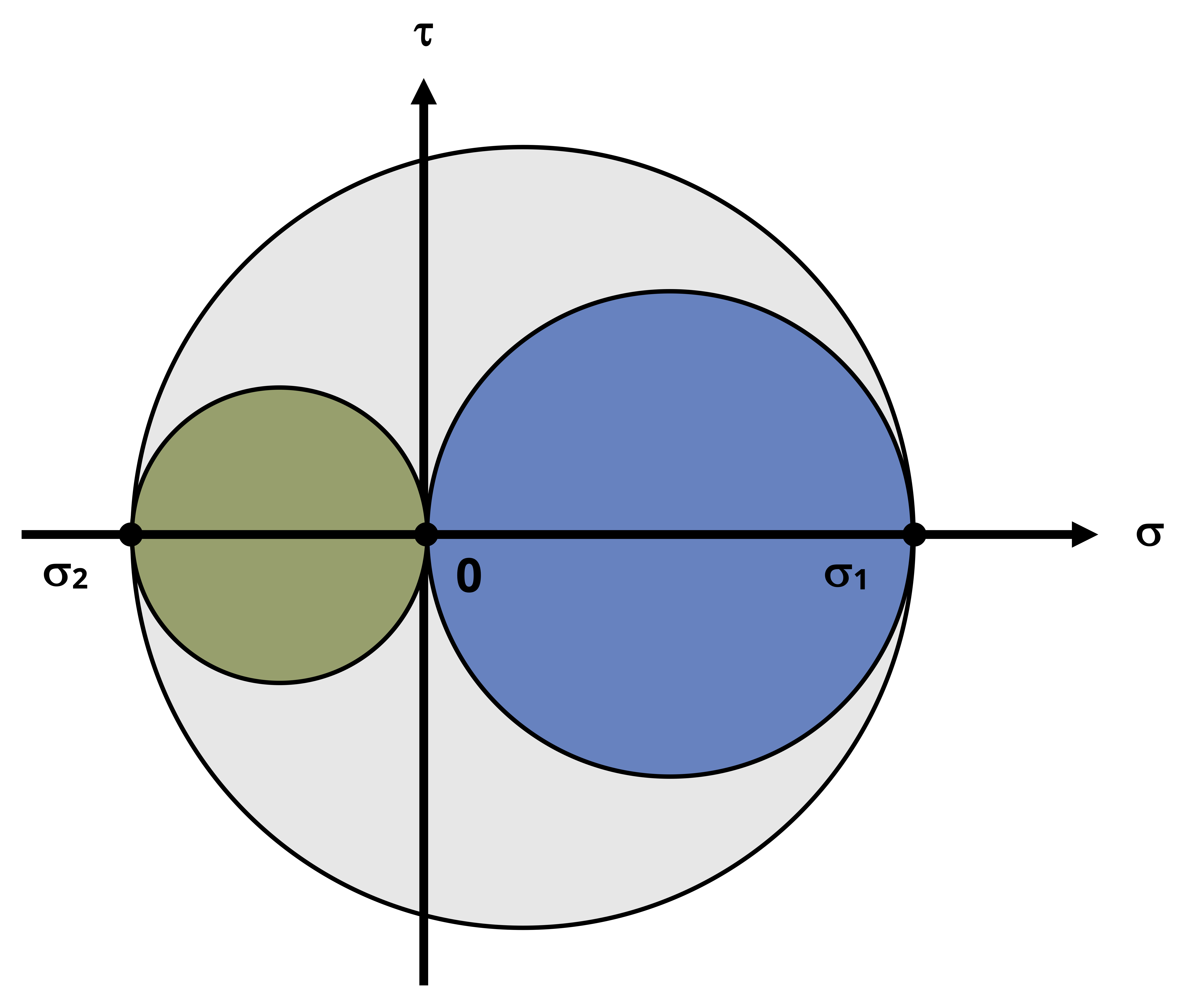
Case 3:
Referring to Figure 12.15, this case is different than the other two because in this case, the Mohr’s circle for the xy plane is the largest circle. This means that the absolute max shear stress and the maximum in-plane shear stress are the same.
So in the case that σ1 and σ2 are opposite in sign, the absolute max shear stress is:
\[ \tau_{(\max )absolute}=\left|\frac{\sigma_1-\sigma_2}{2}\right| \]
More generally, given principal stresses σ1, σ2, and σ3 = 0, the abosulte maximum shear stress can be determined from:
\[ \boxed{\tau_{(\max)absolute}=\left|\frac{\sigma_{\max }-\sigma_{\min }}{2}\right|} \tag{12.4}\]
𝜏(max)absolute = Absolute maximum shear stress [Pa, psi]
𝜎max = Maximum principal stress [Pa, psi]
𝜎min = Minimum principal stress [Pa, psi]
This works for any of the cases above:
Case 1: σmax = σ1, σmin = 0
Case 2: σmax = 0, σmin = σ2
Case 3: σmax = σ1, σmin = σ2
Example 12.4
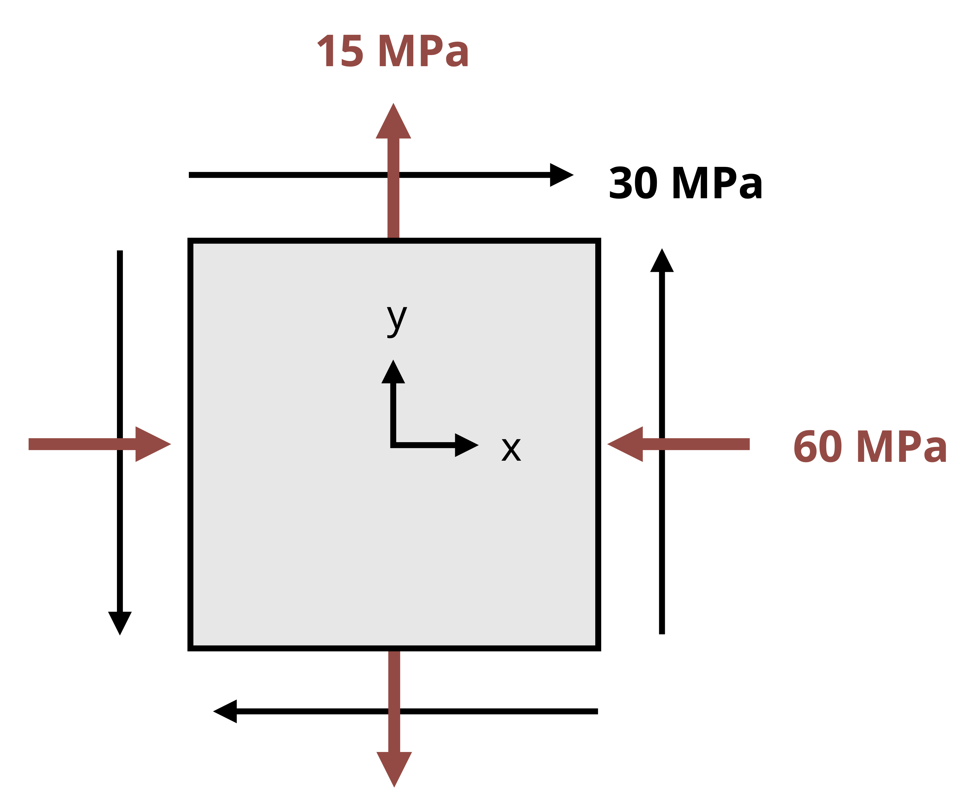
For the stress state given by the stress element below, use Mohr’s Circle to find:
The principal planes and principal stresses. Sketch the stress element rotated to these planes.
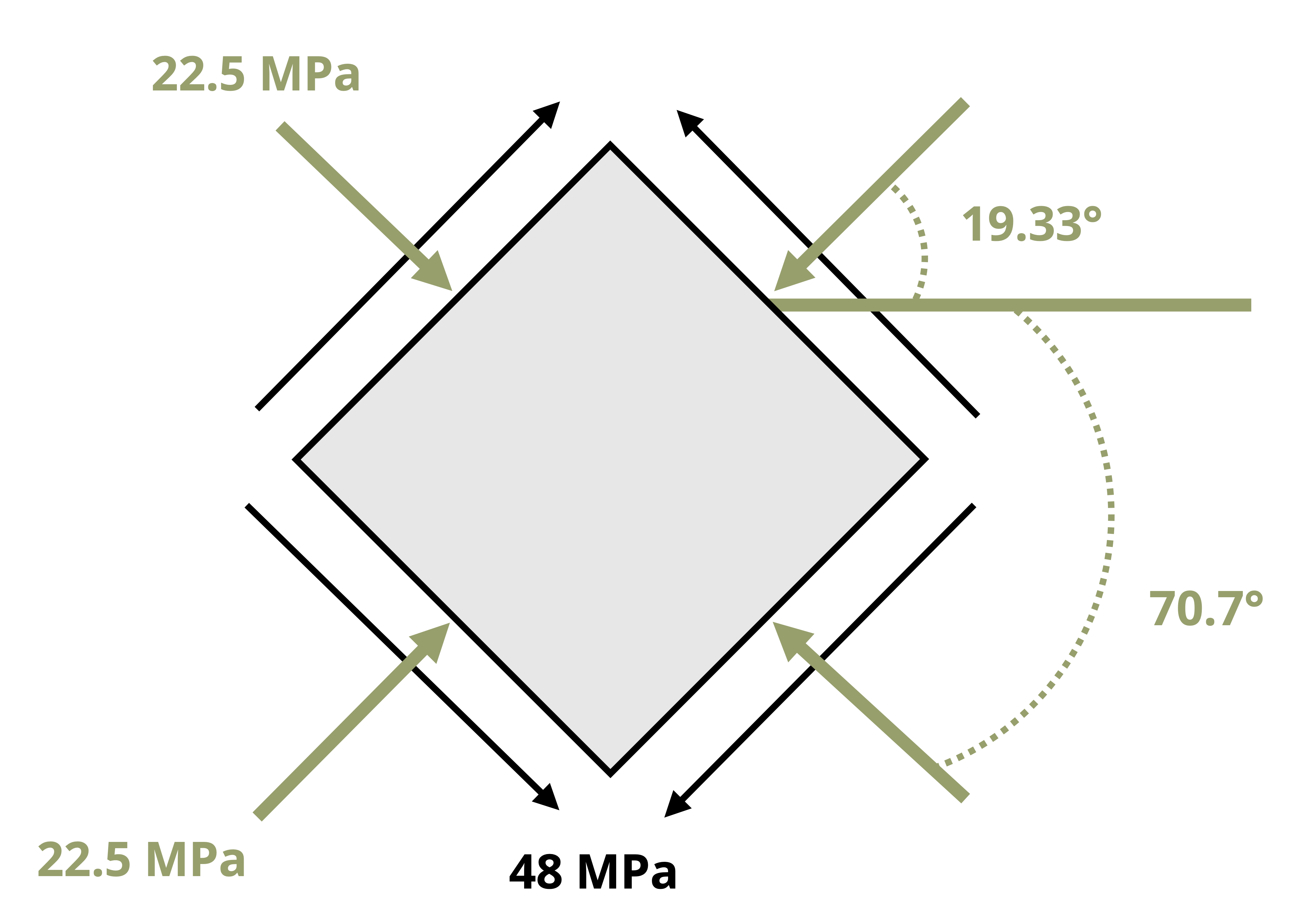
The max in-plane shear stress and the plane at which it acts. Sketch the stress element rotated to this plane.
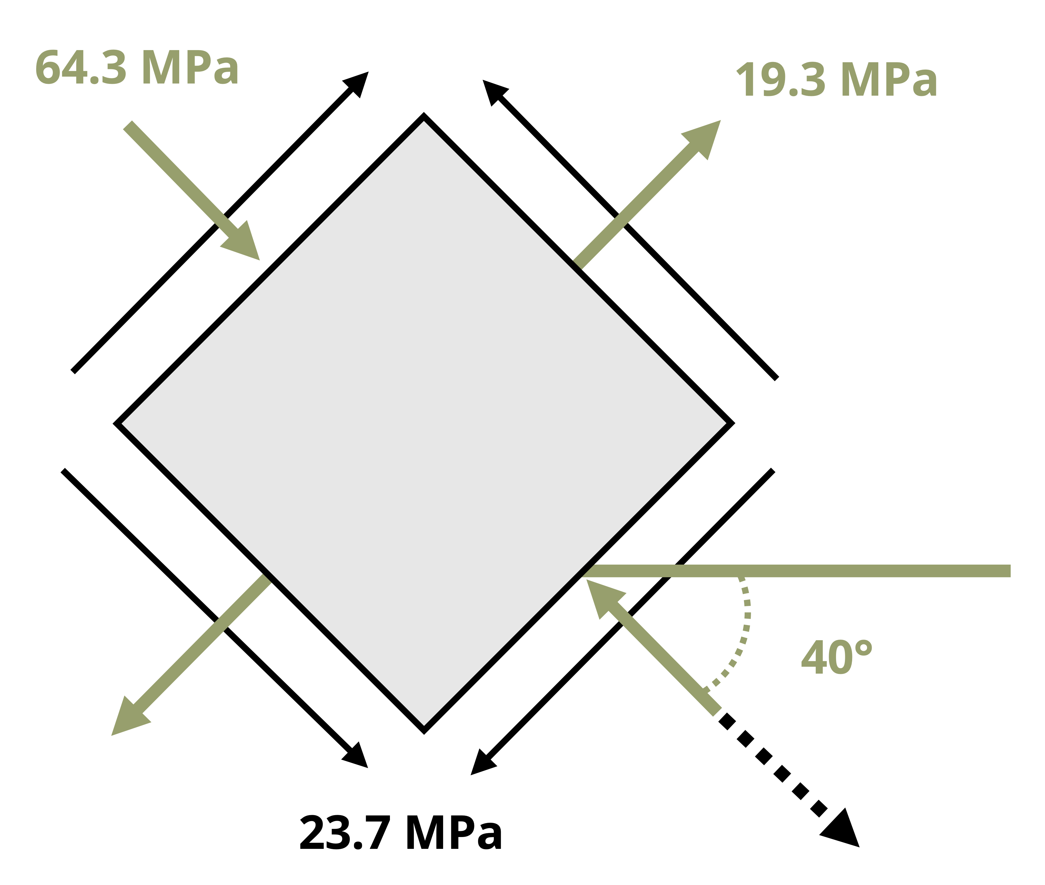
The stress state on the plane on which the stress element is rotated clockwise 40°. Sketch the stress element rotated to this plane.
Example 12.4 demonstrates the use of Mohr’s circle for a stress transformation problem.
Following the steps given in Section 12.3:
The step of drawing the axes will be done as a part of step 3.
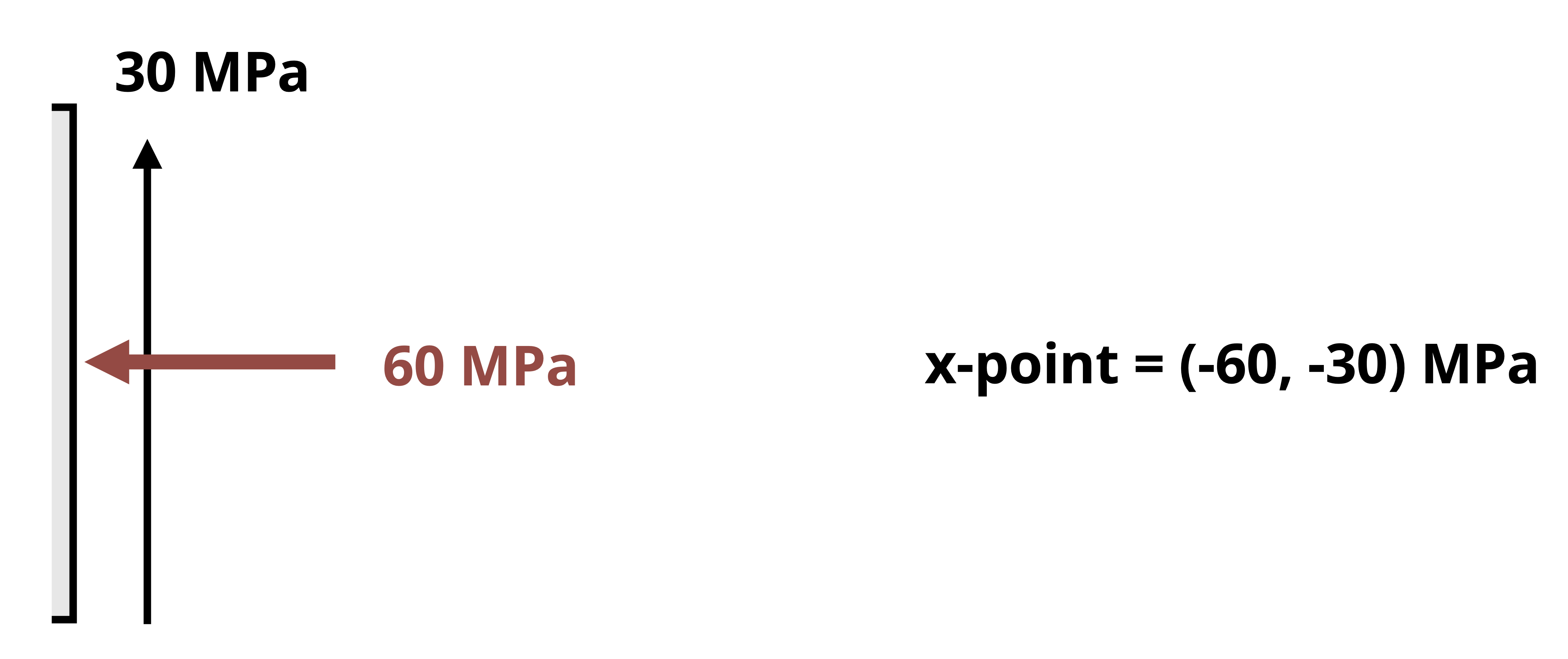
Identify and plot the x-point: Looking at the positive x-face, the normal stress is compressive, so the horizontal coordinate will be -60 MPa. The shear stress arrow is upwards, which would tend to rotate the element counterclockwise, so the vertical coordinate will be negative, or -30 MPa. The x-point is then (-60,-30) MPa
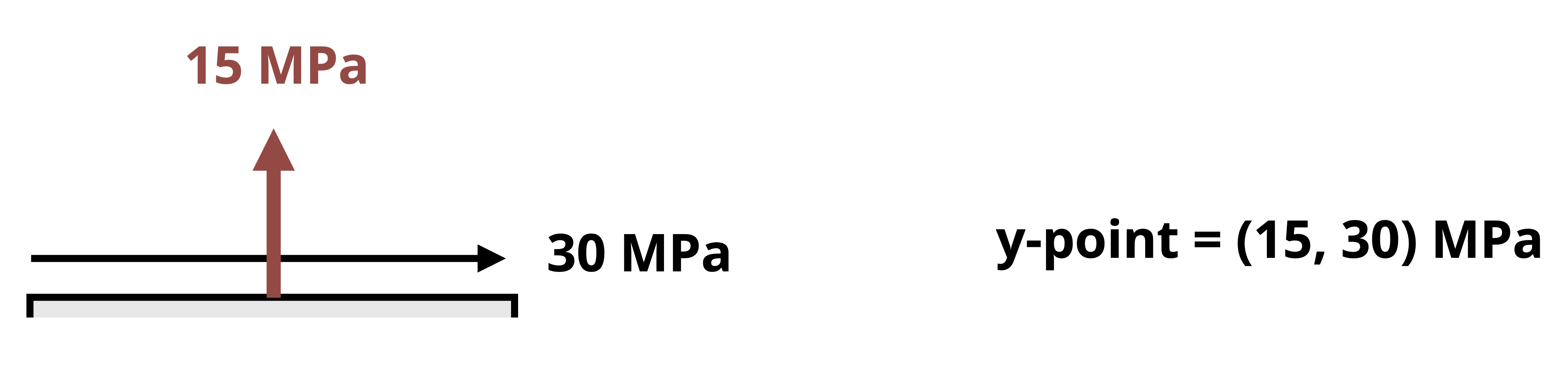
Identify and plot the y-point: Looking at the positive y-face, the normal stress is tensile, so the horizontal coordinate will be +15 MPa. The shear stress arrow is to the right, which would tend to rotate the element clockwise, so the vertical coordinate will be positive, or +30 MPa. The y-point is then (15,30) MPa.
The points are shown plotted in step 3.Connect the two points on the circle and identify the center.
\[ C=\frac{\sigma_x+\sigma_y}{2}=\frac{-60+15}{2}=-22.5 \mathrm{MPa} \]
The radius of the circle is: \(R=\sqrt{\left(\sigma_x-C\right)^2+\tau_{x y}^2}=\sqrt{(-60-(-22.5))^2+30^2}=48.02 \mathrm{MPa}\)
We can now find σ1 by finding the distance from the origin to the rightmost point of the circle on the σ axis. Since C is negative, we can find distance to be C + R = -22.5 MPa + 48.02 MPa = 25.52 MPa.
So σ1 = 25.5 MPa
We can find σ2 by finding the distance from the origin to the leftmost point of the circle on the σ axis. This distance can be expressed as C- R = -48.02 MPa – 22.5 MPa = -70.52 MPa
So σ2 = -70.5 MPa
The max in-plane shear stress is the bottom most point of the circle which is simply R = 48.02 MPa, or τmax (in-plane) = 48.0 MPa.
The normal stress on this plane is C = -22.5 MPa
The principal planes can be found as: \(tan(2\theta_p)=\frac{\sigma_x-C}{\tau_{xy}}=\frac{-60{~MPa}-(-22.5{~MPa})}{30{~MPa}}\)
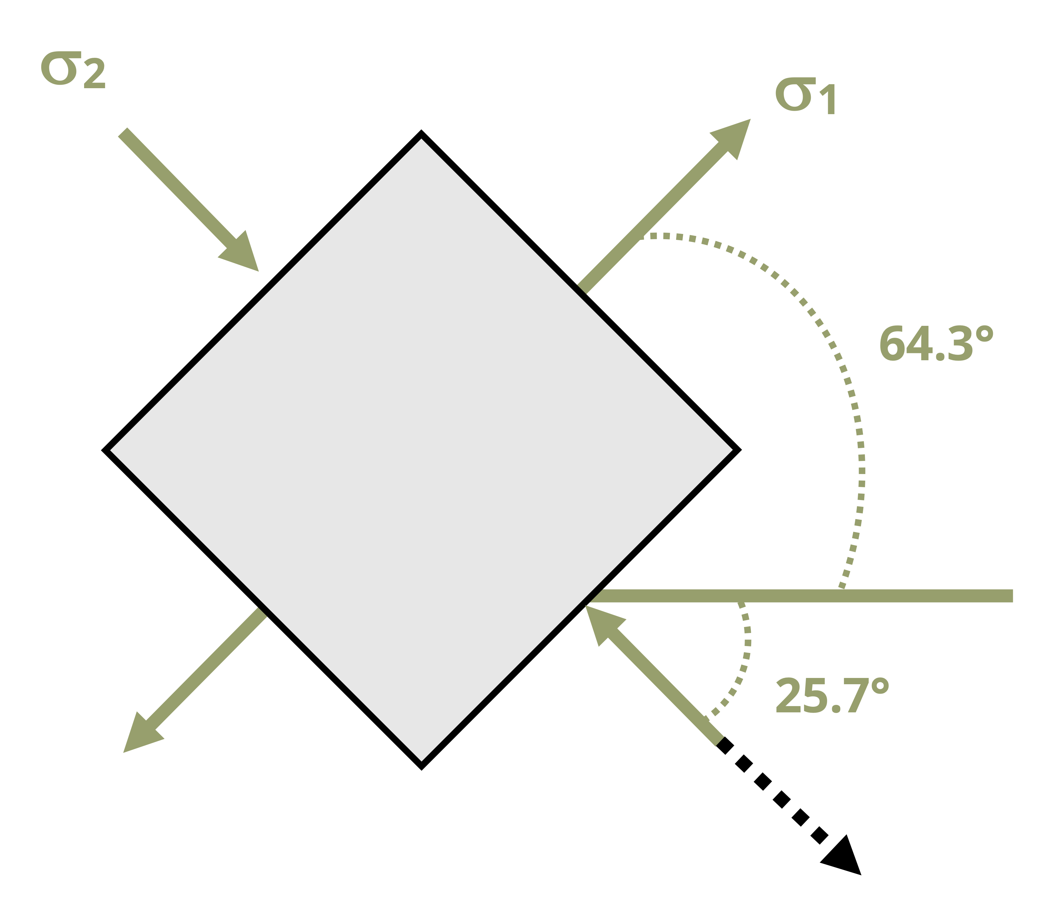
One solution to this equation yields θp = -25.67°. This is the angle of rotation for which σ2 would be shown on the rotated x face. Note the negative angle means this would be a clockwise rotation.The other solution to the equation is that angle plus 90°, which in this case yields θp = 64.33°. This is the angle of rotation for which σ1 would appear on the rotated x-face. The positive angle indicates this would be a counterclockwise rotation.
With the θp angles known, we can see that the 2θs = 90 - 2θp, or θs = 19.33° and -70.67°. In this case, a counterclockwise rotation of the x-point would bring it to the negative side of the vertical axis which corresponds to τmax, so we can say that θs = 19.33° is the plane of max in-plane shear stress.
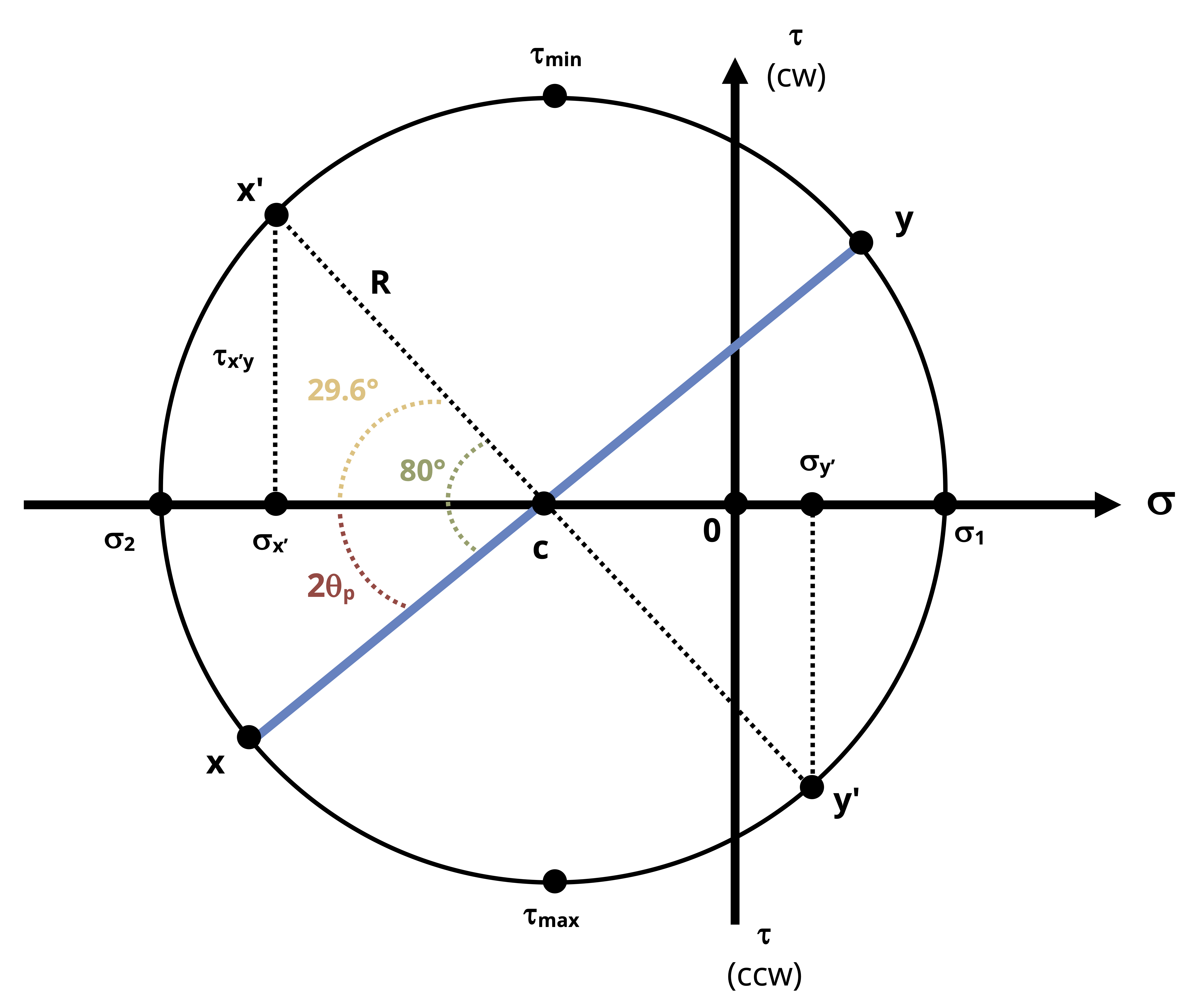
Now we can use Mohr’s Circle to find the stress state on the plane where the stress element is rotated clockwise 40°. The circle is redrawn below for convenience.
Recalling that rotations around the circle are twice the actual rotation, we will draw in a point (denoted as x’) that represents an 80 degree rotation clockwise from the x-point. Since we know from step 7 that the x-point is rotated 2* 25.7° below σ2, we also know that x’ is rotated 80 – 50.4 = 29.6° above σ2.
Since x’ is on the negative σ side and the positive τ side, we know that the normal stress on the x’ face is compressive and the shear stress arrow on the x’ face would tend to rotate the element clockwise (which corresponds to a negative shear stress).We can see from the circle that the shear stress is:
\[ \tau_{x'y'}=-Rsin(29.6^\circ)=-48.08{~MPa}*sin(29.6^\circ)=-23.7{~MPa} \]
and
\[ \sigma_{x'}=C-Rcos(29.6^\circ)=-22.5{~MPa}-48.02{~MPa}*cos(29.6^\circ)=-64.3{~MPa} \]
The stress on the rotated y face, σy’, is obtained by finding the distance from the origin to the y’ point which is directly across the circle from x’.
\[ \sigma_{y'}=C+Rcos(29.6^\circ)=-22.5{~MPa}+48.02{~MPa}*cos(29.6^\circ)=19.3{~MPa} \]
The rotated stress element can be drawn:
σ1 = 25.5 MPa on the principal plane θp = 64.3°
σ2 = -70.5 MPa on the principal plane θp = -25.7°
τmax (in-plane) = 48.0 MPa on the plane θs = 19.33°
On the plane rotated 40° clockwise from the given plane:
σx’ = - 64.3 MPa
σy’ = 19.3 MPa
τx’y’ = -23.7 MPa